
Show code (Load required R packages)
library(tidyverse)
library(glue)
library(lubridate)
library(ggdist)
library(patchwork)
library(cowplot)
library(tinytable)Multi-platform Trace Data Reveal Demographic Differences in Video Game Play, but Individuals Vary Far More
Most knowledge about “who plays (what) video games” comes from surveys subject to recall bias and social desirability effects. Using publicly available behavioral logs from Steam, Xbox, and Nintendo spanning 1.5 million hours from 3768 US and UK adults (18–40 years old), I present a visualization-driven descriptive analysis of how play patterns differ according to age, gender, ethnicity, and neurodiversity. Results uncover a variety of trends that have rarely been observed in public data: among others, that older players’ peak playtime occurs approximately 1 hour earlier in the day, that women tend to re-engage with the same game for a longer time period, and that sports games were more popular among Black, Asian, and neurotypical players than among other ethnic groups and neurodiverse players. Despite intriguing group-level trends, however, within-group variation is far larger: demographic characteristics account for at most 5.4% of gameplay behavioral variation. This work provides an empirically grounded complement to survey research and motivates future investigation into the structural and cultural factors shaping play behavior.
video games, demographics, behavioral data, descriptive, genres
library(tidyverse)
library(glue)
library(lubridate)
library(ggdist)
library(patchwork)
library(cowplot)
library(tinytable)set.seed(8675309)
options(scipen = 999, timeout = 600)
theme_set(theme_minimal())
theme_update(
plot.background = element_rect(fill = "white", color = NA),
panel.background = element_rect(fill = "white", color = NA),
strip.background = element_rect(fill = "black"),
strip.text = element_text(color = "white", size = 10, face = "bold"),
axis.text.y = element_text(color = "black", size = 10),
axis.text.x = element_text(color = "black", size = 10),
panel.grid.minor = element_blank(),
panel.border = element_rect(
colour = "black",
fill = NA,
linewidth = 1
)
)
# Color codebook for consistent theming across all figures
# Each demographic dimension uses a single-hue gradient for easy visual grouping
# Lightest colors are still dark enough to be visible on white backgrounds
# Age: Blues (light to dark with age)
colors_age <- c(
"18-24" = "#9ECAE1",
"25-30" = "#4292C6",
"31-35" = "#2171B5",
"36-40" = "#084594"
)
# Gender: Oranges/reds
colors_gender <- c(
"Man" = "#FD8D3C",
"Woman" = "#D94801",
"Non-binary/Other" = "#7F2704"
)
# Ethnicity: Greens
colors_ethnicity <- c(
"Asian" = "#74C476",
"Black" = "#31A354",
"Mixed/Multiple" = "#006D2C",
"Other" = "#00441B",
"White" = "#002910"
)
# Neurodiversity: Purples
colors_neuro <- c(
"Neurotypical" = "#9E9AC8",
"ADHD" = "#756BB1",
"Autism spectrum" = "#54278F"
)
# Combined list for easy access
demo_colors <- list(
Age = colors_age,
Gender = colors_gender,
Ethnicity = colors_ethnicity,
Neurodiversity = colors_neuro
)
# Helper function to get colors for a demographic dimension
get_demo_colors <- function(demographic) {
demo_colors[[demographic]]
}
# Radar chart theme (for genre profile plots)
theme_radar <- ggplot2::theme_void(base_size = 9) +
theme(
# Make panels pack tightly in patchwork
plot.margin = margin(0, 0, 0, 0, "pt"),
panel.spacing = unit(0, "pt"),
# Titles/subtitles: small, tight vertical footprint
plot.title = element_text(
hjust = 0.5,
size = 9,
face = "bold",
margin = margin(b = 1, unit = "pt")
),
plot.subtitle = element_text(
hjust = 0.5,
size = 7,
colour = "grey40",
margin = margin(b = 0, unit = "pt")
),
# Ensure nothing about backgrounds/axes creates extra grob area
plot.background = element_rect(fill = "white", colour = NA),
panel.background = element_rect(fill = "white", colour = NA),
# Avoid unexpected clipping/margins from titles
plot.title.position = "plot"
)
# Theme for empty placeholder plots (must be *truly* empty and zero-margin)
theme_radar_empty <- ggplot2::theme_void() +
theme(
plot.margin = margin(0, 0, 0, 0, "pt"),
plot.background = element_rect(fill = "white", colour = NA),
panel.background = element_rect(fill = "white", colour = NA)
)
# Theme for header label tiles (Age/Gender/Ethnicity/Neurodiversity)
theme_radar_label <- ggplot2::theme_void(base_size = 10) +
theme(
plot.margin = margin(0, 0, 0, 0, "pt"),
plot.background = element_rect(fill = "white", colour = NA),
panel.background = element_rect(fill = "white", colour = NA)
)
# Load helper functions
source("R/helpers.R")# Download open-play v1.1.0 from Zenodo (cached locally after first download)
zenodo_url <- "https://zenodo.org/records/18430947/files/digital-wellbeing/open-play-v1.1.0.zip?download=1"
zip_path <- "data/open-play-v1.1.0.zip"
if (!file.exists(zip_path)) {
dir.create(dirname(zip_path), showWarnings = FALSE, recursive = TRUE)
options(timeout = max(600, getOption("timeout")))
message("Downloading 194MB file from Zenodo (may take a few minutes)...")
tryCatch(
{
download.file(zenodo_url, zip_path, mode = "wb", method = "libcurl")
message("Download complete!")
},
error = function(e) {
message("Download failed. Please download manually from:")
message(zenodo_url)
message(glue("And save to: {normalizePath(zip_path, mustWork = FALSE)}"))
stop(e)
}
)
}
# Extract zip if not already extracted
extract_dir <- "data/open-play-v1.1.0"
if (!dir.exists(extract_dir)) {
message("Extracting zip archive...")
unzip(zip_path, exdir = "data")
# Rename the extracted folder to a simpler name
extracted_folder <- list.dirs("data", recursive = FALSE, full.names = TRUE)
extracted_folder <- extracted_folder[grepl(
"digital-wellbeing-open-play",
extracted_folder
)]
if (length(extracted_folder) == 1 && extracted_folder != extract_dir) {
file.rename(extracted_folder, extract_dir)
}
}
# Read raw data files
intake <- read_csv(
file.path(extract_dir, "data/clean/survey_intake.csv.gz"),
guess_max = 10000
)
surveys <- read_csv(
file.path(extract_dir, "data/clean/survey_daily.csv.gz")
) |>
filter(pid %in% intake$pid)
xbox <- read_csv(file.path(extract_dir, "data/clean/xbox.csv.gz"))
nintendo <- read_csv(file.path(extract_dir, "data/clean/nintendo.csv.gz"))
steam <- read_csv(
file.path(extract_dir, "data/clean/steam.csv.gz"),
guess_max = 10000
)
games <- read_csv(
file.path(extract_dir, "data/clean/game_metadata.csv.gz"),
guess_max = 10000
)
# Load helper functions from the dataset (includes get_dst_offset for timezone handling)
source(file.path(extract_dir, "R/helpers.R"))# Cache directory for processed telemetry (speeds up re-renders)
cache_dir <- "data/cache"
cache_file <- file.path(cache_dir, "telemetry_cache.rds")
if (file.exists(cache_file)) {
# Load cached objects
message("Loading cached telemetry data...")
cache <- readRDS(cache_file)
sessions_telemetry <- cache$sessions_telemetry
hourly_telemetry <- cache$hourly_telemetry
daily_telemetry <- cache$daily_telemetry
weekly_telemetry <- cache$weekly_telemetry
telemetry_spans <- cache$telemetry_spans
rm(cache)
} else {
message("Processing telemetry data (this may take a few minutes)...")
# Map participants to their local timezone (for DST-aware conversion)
tz_map <- intake |>
mutate(
pid = as.character(pid),
country,
local_timezone,
.keep = "none"
) |>
distinct(pid, .keep_all = TRUE)
# ---------------------------------------------------------------------------
# SESSION-LEVEL (Nintendo + Xbox only; Steam doesn't provide session data)
# ---------------------------------------------------------------------------
sessions_telemetry <- bind_rows(
xbox |> mutate(platform = "Xbox"),
nintendo |> mutate(platform = "Nintendo")
) |>
left_join(tz_map, by = "pid") |>
filter(!is.na(local_timezone)) |>
mutate(
offset_start = get_dst_offset(session_start, country, local_timezone),
offset_end = get_dst_offset(session_end, country, local_timezone),
start_local = session_start + offset_start,
end_local = session_end + offset_end,
duration_min = as.numeric(difftime(
session_end,
session_start,
units = "mins"
))
) |>
filter(
!is.na(session_start),
!is.na(session_end),
session_end > session_start,
duration_min >= 1
)
# ---------------------------------------------------------------------------
# HOURLY (all platforms)
# ---------------------------------------------------------------------------
hourly_from_sessions <- sessions_telemetry |>
filter(!is.na(start_local), !is.na(end_local)) |>
mutate(
h0_local = floor_date(start_local, "hour"),
h1_local = floor_date(end_local - seconds(1), "hour"),
n_hours = as.integer(difftime(h1_local, h0_local, units = "hours")) + 1
) |>
filter(!is.na(n_hours), n_hours > 0) |>
tidyr::uncount(n_hours, .remove = FALSE, .id = "k") |>
mutate(
hour_start_local = h0_local + hours(k - 1),
minutes = pmax(
0,
as.numeric(difftime(
pmin(end_local, hour_start_local + hours(1)),
pmax(start_local, hour_start_local),
units = "mins"
))
),
hour_start_utc = with_tz(hour_start_local, tzone = "UTC")
) |>
select(
pid,
platform,
title_id,
hour_start_local,
hour_start_utc,
minutes
) |>
group_by(pid, platform, title_id, hour_start_local, hour_start_utc) |>
summarise(minutes = sum(minutes, na.rm = TRUE), .groups = "drop")
hourly_from_steam <- steam |>
select(pid, title_id, datetime_hour_start, minutes) |>
mutate(pid = as.character(pid)) |>
left_join(tz_map, by = "pid") |>
filter(!is.na(local_timezone)) |>
mutate(
platform = "Steam",
hour_start_utc = datetime_hour_start,
offset = get_dst_offset(datetime_hour_start, country, local_timezone),
hour_start_local = datetime_hour_start + offset
) |>
select(
pid,
platform,
title_id,
hour_start_local,
hour_start_utc,
minutes
) |>
group_by(pid, platform, title_id, hour_start_local, hour_start_utc) |>
summarise(minutes = sum(minutes, na.rm = TRUE), .groups = "drop")
hourly_telemetry <- bind_rows(hourly_from_sessions, hourly_from_steam)
# ---------------------------------------------------------------------------
# DAILY (aggregated from hourly)
# ---------------------------------------------------------------------------
daily_telemetry <- hourly_telemetry |>
mutate(day_local = as.Date(hour_start_local)) |>
group_by(pid, platform, day_local) |>
summarise(minutes = sum(minutes, na.rm = TRUE), .groups = "drop")
# ---------------------------------------------------------------------------
# WEEKLY (aggregated from daily)
# ---------------------------------------------------------------------------
weekly_telemetry <- daily_telemetry |>
mutate(week = floor_date(day_local, "week")) |>
group_by(pid, platform, week) |>
summarise(minutes = sum(minutes, na.rm = TRUE), .groups = "drop")
# ---------------------------------------------------------------------------
# TELEMETRY SPANS (date ranges per participant/platform)
# ---------------------------------------------------------------------------
telemetry_spans <- daily_telemetry |>
group_by(pid, platform) |>
summarise(
telemetry_start = min(day_local, na.rm = TRUE),
telemetry_end = max(day_local, na.rm = TRUE) + hours(1),
week = floor_date(telemetry_end, "week"),
n_weeks = as.integer(difftime(
telemetry_end,
telemetry_start,
units = "weeks"
)) +
1,
.groups = "drop"
)
# Save to cache
dir.create(cache_dir, showWarnings = FALSE, recursive = TRUE)
saveRDS(
list(
sessions_telemetry = sessions_telemetry,
hourly_telemetry = hourly_telemetry,
daily_telemetry = daily_telemetry,
weekly_telemetry = weekly_telemetry,
telemetry_spans = telemetry_spans
),
cache_file
)
message("Telemetry cache saved to ", cache_file)
}# Clean and collapse demographic variables
demographics <- intake |>
mutate(
pid = as.character(pid),
# Age bins
age_group = cut(
age,
breaks = c(17, 24, 30, 35, 40),
labels = c("18-24", "25-30", "31-35", "36-40")
),
# Gender: collapse to Man / Woman / Non-binary or other
gender_clean = case_when(
gender %in% c("Man", "Male") ~ "Man",
gender %in% c("Woman", "Female") ~ "Woman",
gender == "Prefer not to say" ~ NA_character_,
is.na(gender) ~ NA_character_,
TRUE ~ "Non-binary/Other"
),
# Ethnicity: harmonize UK/US categories
ethnicity_clean = case_when(
ethnicity %in% c("White", "White alone") ~ "White",
ethnicity %in%
c(
"Black",
"Black or African American alone",
"Black, African, Caribbean or Black British"
) ~ "Black",
ethnicity %in%
c("Asian", "Asian alone", "Asian or Asian British") ~ "Asian",
ethnicity %in%
c(
"Mixed",
"Mixed or multiple ethnic groups",
"Two or More Races"
) ~ "Mixed/Multiple",
ethnicity %in% c("Prefer not to say") ~ NA_character_,
is.na(ethnicity) ~ NA_character_,
TRUE ~ "Other"
),
# Neurodiversity: specific categories (identified or diagnosed)
is_neurotypical = neuro_identify == "No",
is_adhd = !is.na(neuro_iden_adhd) | !is.na(neuro_diag_adhd),
is_autism = !is.na(neuro_iden_asd) | !is.na(neuro_diag_asd)
) |>
select(
pid,
country,
age,
age_group,
gender = gender_clean,
ethnicity = ethnicity_clean,
is_neurotypical,
is_adhd,
is_autism
)
# Aggregate weekly playtime to person-level (mean weekly hours across all weeks)
person_playtime <- weekly_telemetry |>
group_by(pid) |>
summarise(
weekly_hours = mean(minutes, na.rm = TRUE) / 60,
total_hours = sum(minutes, na.rm = TRUE) / 60,
n_weeks_observed = n(),
.groups = "drop"
)
# Join demographics to playtime
person_data <- person_playtime |>
left_join(demographics, by = "pid") |>
filter(!is.na(age_group)) # Keep only participants with demographics
# Create long-form dataset for faceted plotting
# Each row = one person × one demographic dimension
# First, create long form for age/gender/ethnicity
demo_long_basic <- person_data |>
pivot_longer(
cols = c(age_group, gender, ethnicity),
names_to = "demographic",
values_to = "group"
) |>
filter(!is.na(group)) |>
select(pid, weekly_hours, total_hours, n_weeks_observed, demographic, group)
# Create long form for neurodiversity (people can appear in multiple categories)
demo_long_neuro <- person_data |>
pivot_longer(
cols = c(is_neurotypical, is_adhd, is_autism),
names_to = "neuro_type",
values_to = "has_condition"
) |>
filter(has_condition == TRUE) |>
mutate(
demographic = "neurodiversity",
group = case_when(
neuro_type == "is_neurotypical" ~ "Neurotypical",
neuro_type == "is_adhd" ~ "ADHD",
neuro_type == "is_autism" ~ "Autism spectrum"
)
) |>
select(pid, weekly_hours, total_hours, n_weeks_observed, demographic, group)
# Combine and set factor levels for display order
person_data_long <- bind_rows(demo_long_basic, demo_long_neuro) |>
mutate(
demographic = factor(
demographic,
levels = c("age_group", "gender", "ethnicity", "neurodiversity"),
labels = c("Age", "Gender", "Ethnicity", "Neurodiversity")
)
)Questions about who plays video games and how play varies across demographic groups remain central to games research and practice. Differences in age, gender, ethnicity, and neurodiversity are routinely invoked to explain variation in genre engagement, time investment, social play, and monetization patterns, with implications for theory development, experimental design, and commercial decision-making.
At the same time, many existing claims about demographic differences in play rest on limited empirical foundations, often relying on self-report data, highly aggregated industry statistics (e.g., Entertainment Software Association, 2025), and/or homogenous samples (Larrieu et al., 2023). Each of these practices seriously limits our understanding of the true differences in behavior among different groups. Researchers have long known that self-report media use data is often a poor reflection of actual digital behavior (Choi et al., 2023; Kahn et al., 2014; e.g., Parry et al., 2021).
Demographic characteristics such as age, gender, and culture are used pervasively across games research and practice, but with varying degrees of empirical grounding. In theory, demographic variables are routinely positioned as moderators of core constructs within theories related to impulse purchasing (Zhang et al., 2021), technology acceptance (Harnadi et al., 2025), social influence (Liu, 2016), and game preferences (González-González et al., 2022), among others—yet such use often treats demographics as proxies for underlying preferences or motivations without specifying the mechanisms through which they operate. In empirical practice, demographics frequently serve as key predictors of outcomes like player types (Santos et al., 2025), esports participation (Kordyaka et al., 2023), or problematic gaming (Lopez-Fernandez et al., 2019), but the practical significance of these associations is rarely scrutinized (Kirk, 1996; Vornhagen et al., 2020). In industry and HCI research, demographic segmentation guides decisions about targeting, content, and design for groups such as women and older players (Gerling et al., 2012; Kaufman et al., 2019), though segmentation based on what players’ recorded behavior is often recognized as more informative (Norman, 2020; Yin et al., 2025). Across all three arenas, the question of how much demographic categories actually explain about individual behavior remains largely unexamined with behavioral data outside of industry internal research.
Digital trace data, defined as behavioral logs automatically collected by digital devices and online platforms, offers a complementary lens. By observing play directly, trace data sidesteps the recall bias and social desirability effects inherent in self-report, while capturing dimensions of play (such as hour-by-hour temporal patterns or engagement span across titles) that surveys cannot feasibly measure. Trace data thus enables more fine-grained descriptions of play and its demographic composition, supports better monitoring of how the characteristics and behaviors of players change over time, and improves predictions about how play and player populations are likely to evolve in the future. The present article marks one such snapshot in the form of a secondary analysis of the Open Play dataset (Ballou et al., 2025)—a large, multi-platform collection of behavioral logs from US and UK adults—to describe how observed play patterns vary across age, gender, ethnicity, and neurodiversity.
In sum, demographic differences are treated as theoretically and practically important, yet the behavioral evidence used to motivate those claims is frequently indirect or coarse. To address this gap, I adopt a descriptive, visualization-first approach that foregrounds both between-group patterns and within-group heterogeneity. I do not conduct null hypothesis significance testing; instead, I focus on the magnitude and structure of observed differences. The work makes two primary contributions:
# Calculate date range for each platform's telemetry
platform_ranges <- daily_telemetry |>
  group_by(platform) |>
  summarise(
    min_date = min(day_local, na.rm = TRUE),
    max_date = max(day_local, na.rm = TRUE),
    .groups = "drop"
  ) |>
  mutate(
    range_text = glue(
      "{format(min_date, '%b %Y')} to {format(max_date, '%b %Y')}"
    )
  )

# Format as a single inline-ready string
telemetry_range_sentence <- platform_ranges |>
  mutate(platform_range = glue("{platform} ({range_text})")) |>
  pull(platform_range) |>
  paste(collapse = ", ")

# Calculate intake survey date range
intake_range <- intake |>
  summarise(
    min_date = min(date, na.rm = TRUE),
    max_date = max(date, na.rm = TRUE)
  )

intake_range_sentence <- glue(
  "{format(intake_range$min_date, '%b %Y')} and {format(intake_range$max_date, '%b %Y')}"
)

games_per_player <- hourly_telemetry |>
  group_by(pid) |>
  summarise(
    n_games = length(unique(title_id))
  ) |>
  pull(n_games) |>
  mean() |>
  round(1)
The data for this study comprise a subset of the data from the Open Play study (Ballou et al., 2025), version 1.1.0. In that study, participants provided access to automated records of their gaming history on one or more platforms (Xbox, Steam, Nintendo Switch, iOS, Android; Xbox is included for US participants only) and completed an intake survey followed by daily and biweekly surveys. The present study uses only the digital trace data from console and PC and demographic data from the intake survey, and does not include daily or biweekly survey data or mobile data (due to lower granularity compared to other trace data streams). Intake surveys were completed between Sep 2024 and Jan 2026. Digital trace data span the following periods: Nintendo (May 2022 to Oct 2025), Steam (Nov 2024 to Oct 2025), Xbox (Apr 2022 to Sep 2025).
Participants were recruited in collaboration with two panel providers, Prolific and PureProfile. Participants were eligible if they were aged 18 or older, resided in the United States or United Kingdom, self-reported playing video games for at least 1 hour per week with at least 50% of their play happening on eligible platforms (Nintendo, Xbox, and Steam), and successfully linked at least one gaming account on Xbox, Steam, and/or Nintendo Switch with validated recent digital trace data.
The procedure for linking gameplay data differed per platform: Steam was collected through a custom platform developed for research purposes, while Xbox and Nintendo data were collected via non-financial data-sharing agreements with the platform owners. An overview of the procedure from the participant perspective is shown in Appendix Table 3, while full details of the recruitment procedures and study methodology are available in (Ballou et al., 2025).
All data and analysis code are available on [repository link removed for anonymous review; anonymized supplementary materials uploaded to PCS].
A description of the sample is shown in Table 1.
Participants in the initial screening sample were quasi-representative; quotas ensured that those screened were approximately nationally representative according to age, gender, and ethnicity. However, the analytic sample is non-representative, as both prevalence of gaming (i.e., likelihood of qualifying for the study) and willingness to participate in the intensive study differed across demographic groups in the screening sample. Nonetheless, the analytic sample consists of a diverse sample across gender and ethnicity.
Particularly noteworthy is the neurodiversity of the sample: 23.8% of participants reported having an ADHD diagnosis, and 16.8% of participants reported having an autism spectrum disorder diagnosis (with 7.4% reporting both)—both far above national averages (see e.g., estimates that 6.0% of US adults have ADHD Staley et al., 2024; and 2.2% of US adults have autism Dietz et al., 2020). While such a high prevalence creates challenges for the generalizability of full-sample analyses, having this degree of diversity present in the sample allows for a more nuanced look at how play patterns vary across different neurotypes, rather than treating neurodivergent players as a monolithic group.
# Analytic sample: participants with trace data who have demographic info
pids_with_telemetry <- daily_telemetry |> distinct(pid) |> pull(pid)

analytic_sample <- demographics |>
  filter(pid %in% pids_with_telemetry, !is.na(age_group))

# Sample sizes by country
n_total <- nrow(analytic_sample)
n_us <- sum(analytic_sample$country == "US")
n_uk <- sum(analytic_sample$country == "UK")

# Build the table
summary_table <- bind_rows(
  # Sample size
  make_table_row(
    "**N**",
    as.character(n_total),
    as.character(n_us),
    as.character(n_uk)
  ),

  # Age
  make_table_row(
    "Age (years)",
    format_mean_sd(analytic_sample$age),
    format_mean_sd(analytic_sample$age[analytic_sample$country == "US"]),
    format_mean_sd(analytic_sample$age[analytic_sample$country == "UK"])
  ),

  # Gender
  make_demo_rows(
    analytic_sample,
    "gender",
    "Gender",
    c("Man", "Woman", "Non-binary/Other"),
    n_total,
    n_us,
    n_uk
  ),

  # Ethnicity
  make_demo_rows(
    analytic_sample,
    "ethnicity",
    "Ethnicity",
    c("White", "Asian", "Black", "Mixed/Multiple", "Other"),
    n_total,
    n_us,
    n_uk
  ),

  # Neurodiversity (non-exclusive, requires manual handling)
  make_table_row("**Neurodiversity**", "", "", ""),
  {
    n_tot <- sum(analytic_sample$is_neurotypical, na.rm = TRUE)
    n_us_val <- sum(
      analytic_sample$is_neurotypical & analytic_sample$country == "US",
      na.rm = TRUE
    )
    n_uk_val <- sum(
      analytic_sample$is_neurotypical & analytic_sample$country == "UK",
      na.rm = TRUE
    )
    make_table_row(
      "    Neurotypical",
      format_n_pct(n_tot, n_total),
      format_n_pct(n_us_val, n_us),
      format_n_pct(n_uk_val, n_uk)
    )
  },
  {
    n_tot <- sum(analytic_sample$is_adhd, na.rm = TRUE)
    n_us_val <- sum(
      analytic_sample$is_adhd & analytic_sample$country == "US",
      na.rm = TRUE
    )
    n_uk_val <- sum(
      analytic_sample$is_adhd & analytic_sample$country == "UK",
      na.rm = TRUE
    )
    make_table_row(
      "    ADHD",
      format_n_pct(n_tot, n_total),
      format_n_pct(n_us_val, n_us),
      format_n_pct(n_uk_val, n_uk)
    )
  },
  {
    n_tot <- sum(analytic_sample$is_autism, na.rm = TRUE)
    n_us_val <- sum(
      analytic_sample$is_autism & analytic_sample$country == "US",
      na.rm = TRUE
    )
    n_uk_val <- sum(
      analytic_sample$is_autism & analytic_sample$country == "UK",
      na.rm = TRUE
    )
    make_table_row(
      "    Autism spectrum",
      format_n_pct(n_tot, n_total),
      format_n_pct(n_us_val, n_us),
      format_n_pct(n_uk_val, n_uk)
    )
  },

  # Platform breakdown
  make_table_row("**Platform**", "", "", ""),
  {
    platform_by_country <- daily_telemetry |>
      distinct(pid, platform) |>
      left_join(analytic_sample |> select(pid, country), by = "pid") |>
      filter(!is.na(country))

    map_dfr(c("Nintendo", "Steam", "Xbox"), function(plat) {
      n_tot <- platform_by_country |> filter(platform == plat) |> nrow()
      n_us_val <- platform_by_country |>
        filter(platform == plat, country == "US") |>
        nrow()
      n_uk_val <- platform_by_country |>
        filter(platform == plat, country == "UK") |>
        nrow()
      make_table_row(
        glue("    {plat}"),
        format_n_pct(n_tot, n_total),
        format_n_pct(n_us_val, n_us),
        format_n_pct(n_uk_val, n_uk)
      )
    })
  }
)

# Identify rows for styling
header_rows <- which(str_detect(summary_table$Characteristic, "^\\*\\*"))
indent_rows <- which(str_detect(summary_table$Characteristic, "^    "))

# Create table
summary_table |>
  tt(
    notes = "Values are M (SD) or N (percent). Neurodiversity categories are non-exclusive."
  ) |>
  format_tt(j = 1, markdown = TRUE) |>
  style_tt(i = header_rows, bold = TRUE) |>
  format_tt(i = header_rows, j = 1, fn = \(x) str_remove_all(x, "\\*\\*")) |>
  style_tt(i = indent_rows, j = 1, indent = 1) |>
  format_tt(i = indent_rows, j = 1, fn = \(x) str_trim(x)) |>
  style_tt(fontsize = 0.8) |>
style_tt(i = 0, bold = TRUE)| Characteristic | Total | US | UK |
|---|---|---|---|
| Values are M (SD) or N (percent). Neurodiversity categories are non-exclusive. | |||
| N | 3768 | 2172 | 1596 |
| Age (years) | 27.1 (5.2) | 26.7 (5) | 27.5 (5.4) |
| Gender | |||
| Man | 2332 (61.9\%) | 1298 (59.8\%) | 1034 (64.8\%) |
| Woman | 1233 (32.7\%) | 740 (34.1\%) | 493 (30.9\%) |
| Non-binary/Other | 198 (5.3\%) | 132 (6.1\%) | 66 (4.1\%) |
| Ethnicity | |||
| White | 2679 (71.1\%) | 1353 (62.3\%) | 1326 (83.1\%) |
| Asian | 323 (8.6\%) | 188 (8.7\%) | 135 (8.5\%) |
| Black | 250 (6.6\%) | 212 (9.8\%) | 38 (2.4\%) |
| Mixed/Multiple | 377 (10\%) | 307 (14.1\%) | 70 (4.4\%) |
| Other | 129 (3.4\%) | 110 (5.1\%) | 19 (1.2\%) |
| Neurodiversity | |||
| Neurotypical | 2158 (57.3\%) | 1201 (55.3\%) | 957 (60\%) |
| ADHD | 898 (23.8\%) | 596 (27.4\%) | 302 (18.9\%) |
| Autism spectrum | 633 (16.8\%) | 345 (15.9\%) | 288 (18\%) |
| Platform | |||
| Nintendo | 1442 (38.3\%) | 789 (36.3\%) | 653 (40.9\%) |
| Steam | 2805 (74.4\%) | 1577 (72.6\%) | 1228 (76.9\%) |
| Xbox | 326 (8.7\%) | 326 (15\%) | 0 (0.0\%) |
The following demographic variables were measured in the intake survey.
Age: Participants entered their age as an integer. Because the multivariate visualizations used here (e.g., radar charts comparing genre profiles) require categorical groupings, continuous age is binned into four groups (18–24, 25–30, 31–35, 36–40) for comparability with the other demographic dimensions.
Gender: Participants selected from the following options: Woman, Man, Non-binary, Prefer to specify, and Prefer not to say. For simplicity, “non-binary” and “prefer to specify” were recoded as “Non-binary/other”.
Ethnicity: Response options were drawn from primary census categories in each respective country. US participants selected between White alone; Black or African American alone; American Indian and Alaska Native alone; Asian alone; Native Hawaiian and Other Pacific Islander alone; Some Other Race alone; and Two or More Races. UK participants selected among White; Mixed or multiple ethnic groups; Asian or Asian British; Black, African, Caribbean or Black British; Other ethnic group; Prefer not to say. For simplicity, I harmonized these categories into a smaller set of labels (e.g., “Black or African American alone” and “Black, African, Caribbean or Black British” were both recoded as “Black”).
Neurodiversity: Participants were asked if they had received a formal diagnosis of neurodiverse conditions from a qualified healthcare professional; if they selected yes, they were provided a list of 12 options. In this paper, I focus solely on players who reported having a diagnosis of either autism spectrum disorder or attention deficit hyperactive disorder, as prevalence of other categories (e.g., dyscalculia) was too small for meaningful analysis.
Gaming behavior on Xbox, Steam, and Nintendo Switch was measured via a mix of (a) session-level data provided by Nintendo of America, Nintendo of Europe, and Microsoft; and (b) hourly playtime collected using open source methods built on the Steam API. The exact data-sharing procedure and data collected varied by platform; details are available in Appendix Table 3, and are described in exhaustive detail in Ballou et al. (2025).
Because Xbox titles are replaced with a random identifier instead of the specific game, subsequent analyses in this paper do not focus on particular games, but rather on genres (as this metadata was provided alongside Xbox games). For reference, the most popular 5 non-Xbox games for each demographic group are shown in Table 4
From the hourly and session-level data, I calculated various summary variables including: total playtime (hours), session count, mean session duration, genre categories (how assigned to titles), title diversity, and hour of day and day of week distributions. These derived variables form the basis of the descriptions to come.
Nintendo and Steam data contain full game titles; to collect game metadata including genres, we used the Internet Games Database (IGDB) API. Xbox data was provided using random identifiers in place of game titles, but with genre labels as seen on the Xbox store. For simplicity, I therefore harmonized IGDB and Xbox genres into a smaller subset of categories (e.g., turn-based strategy, real-time strategy, tactical, MOBA were collapsed into a single “Strategy” category). Full details of the genre mapping are available in the supplementary materials. For the primary genre analysis, each game was assigned to its first listed genre, typically the primary genre; a supplementary multi-genre analysis (Appendix Figure 6) apportioned playtime equally across all genres a game was tagged with and largely replicated the findings.
This study received ethical approval from [redacted for anonymous peer review]. All participants provided informed consent at the start of the study, including consent to their data being shared openly for reanalysis.
Participants were paid at an average rate of £12/hour, equating to: £0.20 for a 1-minute screening, £2 for the 10-minute intake survey (plus £5 for linking at least one account with recent data), £0.80 for each 4-minute daily survey. Participants received a £10 bonus payment for completing at least 24 out of 30 daily surveys.
Results below first depict the behavioral patterns observed in play volume, engagement patterns and temporal organization, and genre composition, before quantifying total explanatory power.
# Calculate per-person session metrics from sessions_telemetry (Nintendo + Xbox only)
person_sessions <- sessions_telemetry |>
  group_by(pid) |>
  summarise(
    n_sessions = n(),
    median_duration = median(duration_min, na.rm = TRUE),
    .groups = "drop"
  ) |>
  left_join(demographics, by = "pid") |>
  filter(!is.na(age_group))

# Combined color palette
all_demo_colors <- c(colors_age, colors_gender, colors_ethnicity, colors_neuro)

# Helper to create a single distribution panel
make_volume_panel <- function(
  data,
  x_var,
  x_label,
  x_scale = "identity",
  x_lim = NULL
) {
  p <- data |>
    ggplot(aes(x = .data[[x_var]], y = group, fill = group)) +
    stat_slabinterval(
      slab_alpha = 0.7,
      point_interval = median_qi,
      interval_color = "black",
      point_color = "black",
      point_size = 1.5,
      scale = 0.85,
      .width = c(0.66, 0.95)
    ) +
    scale_fill_manual(values = all_demo_colors) +
    facet_wrap(~demographic, scales = "free_y", nrow = 1) +
    labs(x = x_label, y = NULL) +
    theme(
      legend.position = "none",
      strip.text = element_text(
        size = 8,
        color = "white",
        margin = margin(t = 2, b = 2)
      ),
      strip.background = element_rect(fill = "black"),
      axis.text.y = element_text(size = 8),
      axis.text.x = element_text(size = 8, angle = 45, hjust = 1),
      panel.spacing.x = unit(12, "pt")
    )

  if (x_scale == "log10") {
    p <- p + scale_x_log10(labels = scales::comma_format())
  }
  if (!is.null(x_lim)) {
    p <- p + coord_cartesian(xlim = x_lim)
  }
  p
}

# Panel A: Weekly hours (from person_data_long)
p_weekly <- make_volume_panel(
  person_data_long,
  "weekly_hours",
  "Mean weekly playtime (hours)",
  x_lim = c(0, 40)
)

# Prepare sessions data in long form
sessions_long_basic <- person_sessions |>
  pivot_longer(
    cols = c(age_group, gender, ethnicity),
    names_to = "demographic",
    values_to = "group"
  ) |>
  filter(!is.na(group)) |>
  select(pid, n_sessions, median_duration, demographic, group)

sessions_long_neuro <- person_sessions |>
  pivot_longer(
    cols = c(is_neurotypical, is_adhd, is_autism),
    names_to = "neuro_type",
    values_to = "has_condition"
  ) |>
  filter(has_condition == TRUE) |>
  mutate(
    demographic = "neurodiversity",
    group = case_when(
      neuro_type == "is_neurotypical" ~ "Neurotypical",
      neuro_type == "is_adhd" ~ "ADHD",
      neuro_type == "is_autism" ~ "Autism spectrum"
    )
  ) |>
  select(pid, n_sessions, median_duration, demographic, group)

sessions_long <- bind_rows(sessions_long_basic, sessions_long_neuro) |>
  mutate(
    demographic = factor(
      demographic,
      levels = c("age_group", "gender", "ethnicity", "neurodiversity"),
      labels = c("Age", "Gender", "Ethnicity", "Neurodiversity")
    )
  )

# Panel B: Session count
p_sessions <- make_volume_panel(
  sessions_long,
  "n_sessions",
  "Total sessions (log scale)",
  x_scale = "log10",
  x_lim = c(10, 5000)
)

# Panel C: Session duration
p_duration <- make_volume_panel(
  sessions_long,
  "median_duration",
  "Median session duration (minutes)",
  x_lim = c(0, 120)
)

# Combine vertically with A/B/C labels
p_weekly /
  p_sessions /
  p_duration +
  plot_annotation(tag_levels = "A") &
  theme(plot.tag = element_text(face = "bold", size = 12))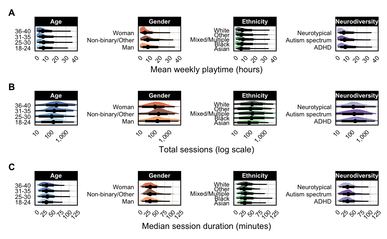
# Gender comparisons (weekly hours)
gender_hours <- person_data_long |>
  filter(demographic == "Gender") |>
  group_by(group) |>
  summarise(median_hours = median(weekly_hours, na.rm = TRUE), .groups = "drop")

hours_women <- gender_hours |> filter(group == "Woman") |> pull(median_hours)
hours_men <- gender_hours |> filter(group == "Man") |> pull(median_hours)
hours_women_fmt <- sprintf("%.1f", hours_women)
hours_men_fmt <- sprintf("%.1f", hours_men)

# Neurodiversity comparisons (sessions and duration)
neuro_sessions <- sessions_long |>
  filter(demographic == "Neurodiversity") |>
  group_by(group) |>
  summarise(
    median_sessions = median(n_sessions, na.rm = TRUE),
    median_duration = median(median_duration, na.rm = TRUE),
    .groups = "drop"
  )

sessions_adhd <- neuro_sessions |>
  filter(group == "ADHD") |>
  pull(median_sessions)
sessions_neurotypical <- neuro_sessions |>
  filter(group == "Neurotypical") |>
  pull(median_sessions)
duration_adhd <- neuro_sessions |>
  filter(group == "ADHD") |>
  pull(median_duration)
duration_neurotypical <- neuro_sessions |>
  filter(group == "Neurotypical") |>
  pull(median_duration)

sessions_adhd_fmt <- scales::comma(round(sessions_adhd))
sessions_neurotypical_fmt <- scales::comma(round(sessions_neurotypical))
duration_adhd_fmt <- sprintf("%.0f", duration_adhd)
duration_neurotypical_fmt <- sprintf("%.0f", duration_neurotypical)
Figure 1 visualizes the typical weekly playtime (Panel A, top row), total recorded sessions (Panel B, middle row), and typical session duration (Panel C, bottom row) for each group. The heavily overlapping histograms across groups indicate that group differences account for very little variation in playtime: in the sample, most groups showed similar distributions of play volume.
A few trends nonetheless emerge: women played fewer weekly hours than men (5.2 vs 8.1 mean hours). There is a small observed difference in the total number of sessions played by participants with ADHD compared to neurotypical players (169 vs 128), but no difference in median session duration (31 vs 31 minutes). Asian players in the sample had slightly lower playtime and sessions than other ethnic groups.
# Calculate per-game engagement metrics
game_engagement <- hourly_telemetry |>
  mutate(day_local = as.Date(hour_start_local)) |>
  group_by(pid, title_id) |>
  summarise(
    first_day = min(day_local, na.rm = TRUE),
    last_day = max(day_local, na.rm = TRUE),
    total_hours = sum(minutes, na.rm = TRUE) / 60,
    n_days = n_distinct(day_local),
    .groups = "drop"
  ) |>
  mutate(engagement_span = as.numeric(last_day - first_day))

# Filter to sticky games (2+ days)
sticky_games <- game_engagement |>
  filter(n_days >= 2)

# Person-level medians
person_engagement <- sticky_games |>
  group_by(pid) |>
  summarise(
    median_span = median(engagement_span, na.rm = TRUE),
    median_hours = median(total_hours, na.rm = TRUE),
    .groups = "drop"
  ) |>
  left_join(demographics, by = "pid") |>
  filter(!is.na(age_group))

# Long-form for engagement
engagement_long_basic <- person_engagement |>
  pivot_longer(
    cols = c(age_group, gender, ethnicity),
    names_to = "demographic",
    values_to = "group"
  ) |>
  filter(!is.na(group)) |>
  select(pid, median_span, median_hours, demographic, group)

engagement_long_neuro <- person_engagement |>
  pivot_longer(
    cols = c(is_neurotypical, is_adhd, is_autism),
    names_to = "neuro_type",
    values_to = "has_condition"
  ) |>
  filter(has_condition == TRUE) |>
  mutate(
    demographic = "neurodiversity",
    group = case_when(
      neuro_type == "is_neurotypical" ~ "Neurotypical",
      neuro_type == "is_adhd" ~ "ADHD",
      neuro_type == "is_autism" ~ "Autism spectrum"
    )
  ) |>
  select(pid, median_span, median_hours, demographic, group)

engagement_long <- bind_rows(engagement_long_basic, engagement_long_neuro)

engagement_summary <- engagement_long |>
  group_by(demographic, group) |>
  summarise(
    median_span = median(median_span, na.rm = TRUE),
    median_hours = median(median_hours, na.rm = TRUE),
    .groups = "drop"
  )

all_demo_colors <- c(colors_age, colors_gender, colors_ethnicity, colors_neuro)

engagement_summary |>
  ggplot(aes(x = median_span, y = median_hours, color = group, label = group)) +
  geom_point(size = 3) +
  ggrepel::geom_text_repel(
    size = 2.8,
    max.overlaps = 20,
    segment.color = "grey60",
    segment.size = 0.3,
    box.padding = 0.5,
    point.padding = 0.4,
    min.segment.length = 0.1,
    force = 2
  ) +
  scale_color_manual(values = all_demo_colors) +
  labs(
    x = "Median engagement span (days)",
    y = "Median hours per game"
  ) +
  theme(legend.position = "none")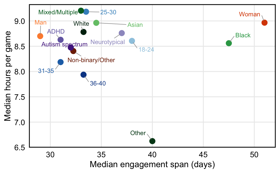
Figure 2 shows difference in engagement tendencies, with engagement span (i.e., the median time between the first and last recorded session of a game, for games with recorded sessions on at least 2 separate days) on the x-axis, and median hours played per distinct game on the y-axis. The upper left represents groups that spend more time in a typical game and concentrate this time into a shorter period, whereas the bottom right represents groups that play less of a particular game, and spread this time out over a longer period.
Results show only small differences in engagement time, with most groups playing between 7.9 and 9.2 hours before moving onto another game. Black and women players tend to spread their engagement out over a longer period, with a typical game being played for approximately 50 days, whereas men and most other groups tend to play a game between 29 and 40 days.
# Panel A: Time of day by age group
hourly_by_age <- hourly_telemetry |>
  mutate(hour = hour(hour_start_local)) |>
  left_join(demographics |> select(pid, age_group), by = "pid") |>
  filter(!is.na(age_group)) |>
  group_by(age_group, hour) |>
  summarise(total_minutes = sum(minutes, na.rm = TRUE), .groups = "drop") |>
  group_by(age_group) |>
  mutate(prop = total_minutes / sum(total_minutes)) |>
  ungroup()

p_time_of_day <- hourly_by_age |>
  ggplot(aes(x = hour, y = prop, color = age_group, group = age_group)) +
  geom_line(linewidth = 1) +
  geom_point(size = 1.5) +
  scale_x_continuous(
    breaks = seq(0, 23, by = 6),
    labels = c("12am", "6am", "12pm", "6pm")
  ) +
  scale_y_continuous(labels = scales::percent_format()) +
  scale_color_manual(values = colors_age) +
  labs(
    x = "Hour of day",
    y = "Proportion of playtime",
    color = "Age"
  ) +
  theme(
    legend.position = "bottom",
    legend.title = element_text(size = 8),
    legend.text = element_text(size = 7)
  ) +
  guides(color = guide_legend(nrow = 1))

# Panel B: Routine vs weekend concentration
calc_top3_share <- function(mins_by_hour) {
  if (sum(mins_by_hour) == 0) {
    return(NA_real_)
  }
  sorted <- sort(mins_by_hour, decreasing = TRUE)
  sum(sorted[1:min(3, length(sorted))]) / sum(sorted)
}

person_temporal <- hourly_telemetry |>
  mutate(
    hour = hour(hour_start_local),
    day_local = as.Date(hour_start_local),
    dow = wday(day_local, week_start = 1),
    is_weekend = dow >= 6
  ) |>
  group_by(pid) |>
  summarise(
    top3_share = {
      hour_mins <- tapply(minutes, hour, sum, default = 0)
      calc_top3_share(hour_mins)
    },
    weekend_mins = sum(minutes[is_weekend], na.rm = TRUE),
    weekday_mins = sum(minutes[!is_weekend], na.rm = TRUE),
    total_mins = weekend_mins + weekday_mins,
    weekend_prop = weekend_mins / total_mins,
    .groups = "drop"
  ) |>
  filter(total_mins > 60, !is.na(top3_share)) |>
  left_join(demographics, by = "pid") |>
  filter(!is.na(age_group))

temporal_long_basic <- person_temporal |>
  pivot_longer(
    cols = c(age_group, gender, ethnicity),
    names_to = "demographic",
    values_to = "group"
  ) |>
  filter(!is.na(group)) |>
  select(pid, top3_share, weekend_prop, demographic, group)

temporal_long_neuro <- person_temporal |>
  pivot_longer(
    cols = c(is_neurotypical, is_adhd, is_autism),
    names_to = "neuro_type",
    values_to = "has_condition"
  ) |>
  filter(has_condition == TRUE) |>
  mutate(
    demographic = "neurodiversity",
    group = case_when(
      neuro_type == "is_neurotypical" ~ "Neurotypical",
      neuro_type == "is_adhd" ~ "ADHD",
      neuro_type == "is_autism" ~ "Autism spectrum"
    )
  ) |>
  select(pid, top3_share, weekend_prop, demographic, group)

temporal_long <- bind_rows(temporal_long_basic, temporal_long_neuro)

temporal_summary <- temporal_long |>
  group_by(demographic, group) |>
  summarise(
    median_top3 = median(top3_share, na.rm = TRUE),
    median_weekend = median(weekend_prop, na.rm = TRUE),
    .groups = "drop"
  )

p_routine_weekend <- temporal_summary |>
  ggplot(aes(
    x = median_top3,
    y = median_weekend,
    color = group,
    label = group
  )) +
  geom_point(size = 3) +
  ggrepel::geom_text_repel(
    size = 2.5,
    max.overlaps = 20,
    segment.color = "grey60",
    segment.size = 0.3,
    box.padding = 0.5,
    point.padding = 0.4,
    min.segment.length = 0.1,
    force = 2
  ) +
  scale_color_manual(values = all_demo_colors) +
  scale_x_continuous(labels = scales::percent_format()) +
  scale_y_continuous(labels = scales::percent_format()) +
  labs(
    x = "Routine concentration\n(% play in top 3 hours)",
    y = "Weekend concentration"
  ) +
  theme(legend.position = "none")

# Combine panels
p_time_of_day +
  p_routine_weekend +
  plot_annotation(tag_levels = "A") &
  theme(plot.tag = element_text(face = "bold", size = 12))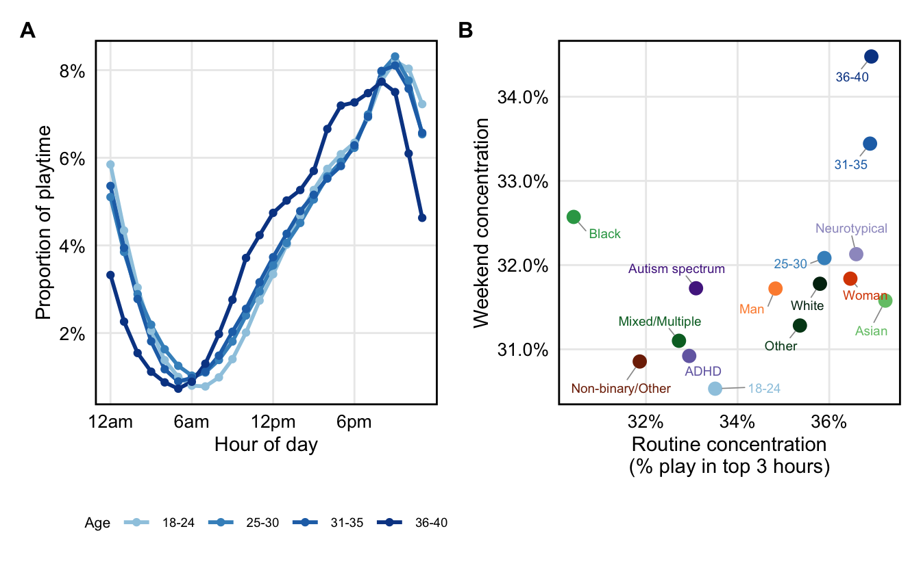
Next, I assessed how the time of play differs across demographic groups in the sample. For each user, I calculated the proportion of total playtime taking place in each of 24 hourly bins, after converting session timestamps to local timezones. I further calculated the proportion of playtime taking place on weekdays vs weekends, and the percentage of play that takes place during a given person’s top 3 hours. The latter constitutes an index of play routine and stability (for example, someone plays exclusively between 6–9pm would have a value of 100%, whereas someone who plays equally throughout the 24-hour would have a value of 3/24 = 12.5%).
# Extract values from temporal_summary (computed in fig-temporal chunk)
weekend_18_24 <- temporal_summary |>
  filter(group == "18-24") |>
  pull(median_weekend) *
  100
weekend_36_40 <- temporal_summary |>
  filter(group == "36-40") |>
  pull(median_weekend) *
  100
routine_18_24 <- temporal_summary |>
  filter(group == "18-24") |>
  pull(median_top3) *
  100
routine_36_40 <- temporal_summary |>
  filter(group == "36-40") |>
  pull(median_top3) *
  100
routine_asian <- temporal_summary |>
  filter(group == "Asian") |>
  pull(median_top3) *
  100
routine_black <- temporal_summary |>
  filter(group == "Black") |>
  pull(median_top3) *
  100

weekend_18_24_fmt <- sprintf("%.1f", weekend_18_24)
weekend_36_40_fmt <- sprintf("%.1f", weekend_36_40)
routine_18_24_fmt <- sprintf("%.1f", routine_18_24)
routine_36_40_fmt <- sprintf("%.1f", routine_36_40)
routine_asian_fmt <- sprintf("%.1f", routine_asian)
routine_black_fmt <- sprintf("%.1f", routine_black)
Results (Figure 3, Panel A) show that 18–35 year olds have similar play patterns, with 9pm being the peak gaming hour. Playtime among 36-40 year-olds shifts slightly earlier, peaking at 8pm.
Figure 3 Panel B shows routine and weekend concentration for each demographic group. In the present sample, older players concentrated their play on weekends more than younger groups (30.5% of play taking place on weekends for 18–24 year olds vs 34.5% for 36–40 year olds) and had more fixed routines (33.5% of 18–24 year olds’ play took place within their top 3 hours, compared to 36.9% for 36–40 year olds). Among ethnic backgrounds, Asian players had the most stable play routines, whereas Black players were least concentrated in consistent times of day (30.4% of playtime falling in the top 3 hours for Black players, 37.2% for Asian players).
# -----------------------------------------------------------------------------
# PRIMARY GENRE MAPPING (first-listed genre only)
# -----------------------------------------------------------------------------
games_genres_primary <- games |>
  mutate(
    genre_raw = str_extract(genres, "^[^,]+") |> str_trim(),
    genre_clean = clean_genre(genre_raw)
  ) |>
  filter(!is.na(genre_clean)) |>
  distinct(original_name, genre_clean)

# -----------------------------------------------------------------------------
# MULTI-GENRE MAPPING (games assigned to all listed genres, time apportioned)
# -----------------------------------------------------------------------------
games_genres_multi <- games |>
  filter(!is.na(genres)) |>
  separate_rows(genres, sep = ",\\s*") |>
  mutate(genre_clean = clean_genre(genres)) |>
  filter(!is.na(genre_clean)) |>
  distinct(original_name, genre_clean) |>
  group_by(original_name) |>
  mutate(genre_weight = 1 / n()) |>
  ungroup()

# -----------------------------------------------------------------------------
# PRIMARY GENRE DATA (for main radar chart)
# -----------------------------------------------------------------------------
genre_playtime_primary <- hourly_telemetry |>
  left_join(games_genres_primary, by = c("title_id" = "original_name")) |>
  filter(!is.na(genre_clean)) |>
  left_join(demographics, by = "pid") |>
  filter(!is.na(age_group))

genre_by_demo_primary <- genre_playtime_primary |>
  group_by(
    pid,
    genre_clean,
    age_group,
    gender,
    ethnicity,
    is_neurotypical,
    is_adhd,
    is_autism
  ) |>
  summarise(minutes = sum(minutes, na.rm = TRUE), .groups = "drop")

# Abbreviate long genre names for display
abbreviate_genre <- function(x) {
  case_when(
    x == "Role-playing (RPG)" ~ "RPG",
    x == "Simulator" ~ "Simulation",
    TRUE ~ x
  )
}

# Top genres by total playtime (used for both versions)
top_genres <- genre_by_demo_primary |>
  group_by(genre_clean) |>
  summarise(total = sum(minutes), .groups = "drop") |>
  slice_max(total, n = 8) |>
  mutate(genre_clean = abbreviate_genre(genre_clean)) |>
  pull(genre_clean)

# Apply abbreviation to base data before computing proportions
genre_by_demo_primary <- genre_by_demo_primary |>
  mutate(genre_clean = abbreviate_genre(genre_clean))

genre_props_primary <- build_genre_props(genre_by_demo_primary)

# Calculate deviation on ALL genres first, then filter for display
genre_props_dev_primary <- calc_genre_deviation(
  genre_by_demo_primary,
  genre_props_primary
)

genre_props_dev_plot_primary <- genre_props_dev_primary |>
  filter(genre_clean %in% top_genres) |>
  mutate(genre_clean = factor(genre_clean, levels = top_genres))

group_ns_primary <- calc_group_ns(genre_by_demo_primary)

# -----------------------------------------------------------------------------
# MULTI-GENRE DATA (for appendix radar chart)
# Playtime is apportioned equally across all genres a game belongs to
# -----------------------------------------------------------------------------
genre_playtime_multi <- hourly_telemetry |>
  left_join(
    games_genres_multi,
    by = c("title_id" = "original_name"),
    relationship = "many-to-many"
  ) |>
  filter(!is.na(genre_clean)) |>
  # Apply weight to apportion playtime across genres
  mutate(minutes_weighted = minutes * genre_weight) |>
  left_join(demographics, by = "pid") |>
  filter(!is.na(age_group))

genre_by_demo_multi <- genre_playtime_multi |>
  group_by(
    pid,
    genre_clean,
    age_group,
    gender,
    ethnicity,
    is_neurotypical,
    is_adhd,
    is_autism
  ) |>
  summarise(minutes = sum(minutes_weighted, na.rm = TRUE), .groups = "drop") |>
  # Apply abbreviation to base data before computing proportions
  mutate(genre_clean = abbreviate_genre(genre_clean))

genre_props_multi <- build_genre_props(genre_by_demo_multi)

# Calculate deviation on ALL genres first, then filter for display
# (filtering before deviation calculation breaks leave-one-out math)
genre_props_dev_multi <- calc_genre_deviation(
  genre_by_demo_multi,
  genre_props_multi
)

genre_props_dev_plot_multi <- genre_props_dev_multi |>
  filter(genre_clean %in% top_genres) |>
  mutate(genre_clean = factor(genre_clean, levels = top_genres))

group_ns_multi <- calc_group_ns(genre_by_demo_multi)# Use pre-calculated deviation (computed on all genres, then filtered for display)
build_radar_grid(
genre_props_dev_plot_primary,
group_ns_primary,
top_genres,
demo_colors,
theme_radar,
theme_radar_empty,
theme_radar_label
)
# Count unique raw genres before simplification
n_raw_genres <- games |>
filter(!is.na(genres)) |>
separate_rows(genres, sep = ",\\s*") |>
distinct(genres) |>
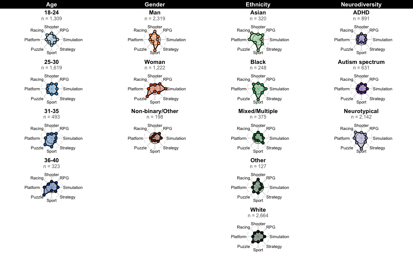
nrow()To visualize differences in genre preferences, I calculated the sum of each user’s playtime taking place in each of the 8 genres within the simplified genre taxonomy described in the measure section (raw play proportions for all 23 genres in the unsimplified data can be found in Appendix Table 5).
Results (Figure 4) visualizes these results. Each demographic group is a radar; the grey circle represents average genre allocation for all other groups (i.e., for 18-24 year olds, the grey line represents the average genre allocation across all age groups, 25–40). The outer dashed line represents 200% of that average, and the inner dashed ring represents 50%. Points farther from the center therefore indicate that this genre is relatively popular among that demographic group, whereas points closer to the center indicate that the genre is relatively unpopular.
A wide variety of observed differences emerge. Among other differences, results in the present sample align with well-documented preferences among men for sports games, and among women for puzzle and simulation games. Asian players in the sample played relatively high amounts of racing, platform, and sports games, whereas White players played slightly more puzzle games than other ethnic groups. Neurodiverse players had slight preference for RPGs compared to neurotypical players, who played more racing games.
# Create simplified neurodiversity variable
demographics_intersect <- demographics |>
  mutate(
    neuro_simple = case_when(
      is_neurotypical ~ "Neurotypical",
      is_adhd | is_autism ~ "Neurodiverse",
      TRUE ~ NA_character_
    )
  )

# Prepare base data with abbreviated genres
base_data <- genre_playtime_primary |>
  left_join(demographics_intersect |> select(pid, neuro_simple), by = "pid") |>
  filter(!is.na(neuro_simple), !is.na(gender), !is.na(ethnicity)) |>
  mutate(genre_clean = abbreviate_genre(genre_clean)) |>
  filter(genre_clean %in% top_genres)

# Step 1: Total minutes by genre (across entire dataset)
genre_totals <- base_data |>
  group_by(genre_clean) |>
  summarise(total_genre_min = sum(minutes, na.rm = TRUE), .groups = "drop")

grand_total <- sum(genre_totals$total_genre_min)

# Step 2: Minutes by intersection × genre
intersect_genre <- base_data |>
  group_by(age_group, gender, ethnicity, neuro_simple, genre_clean) |>
  summarise(int_genre_min = sum(minutes, na.rm = TRUE), .groups = "drop")

# Step 3: Total minutes by intersection (sum across genres)
intersect_totals <- intersect_genre |>
  group_by(age_group, gender, ethnicity, neuro_simple) |>
  summarise(int_total_min = sum(int_genre_min), .groups = "drop")

# Step 4: Sample sizes
intersect_n <- base_data |>
  distinct(pid, age_group, gender, ethnicity, neuro_simple) |>
  count(age_group, gender, ethnicity, neuro_simple, name = "n")

# Step 5: Filter to n >= 75
valid_n <- intersect_n |> filter(n >= 60)

# Step 6: Calculate leave-one-out ratios
intersect_props <- intersect_genre |>
  inner_join(
    valid_n,
    by = c("age_group", "gender", "ethnicity", "neuro_simple")
  ) |>
  inner_join(
    intersect_totals,
    by = c("age_group", "gender", "ethnicity", "neuro_simple")
  ) |>
  inner_join(genre_totals, by = "genre_clean") |>
  mutate(
    # This intersection's proportion in this genre
    int_prop = int_genre_min / int_total_min,
    # Everyone ELSE's minutes in this genre
    others_genre_min = total_genre_min - int_genre_min,
    others_total_min = grand_total - int_total_min,
    # Everyone else's proportion
    others_prop = others_genre_min / others_total_min,
    # Ratio: intersection vs others (>1 means over-representation)
    ratio = int_prop / others_prop,
    log_ratio = log2(ratio),
    log_ratio_capped = pmin(pmax(log_ratio, -1), 1)
  )

# Create factor levels for ordered display
intersect_plot <- intersect_props |>
  mutate(
    age_group = factor(
      age_group,
      levels = c("18-24", "25-30", "31-35", "36-40")
    ),
    gender = factor(gender, levels = c("Man", "Woman", "Non-binary/Other")),
    ethnicity = factor(
      ethnicity,
      levels = c("Asian", "Black", "Mixed/Multiple", "Other", "White")
    ),
    neuro_simple = factor(
      neuro_simple,
      levels = c("Neurotypical", "Neurodiverse")
    ),
    label = glue("{age_group}, {gender}, {ethnicity}, {neuro_simple} (n={n})")
  ) |>
  arrange(age_group, gender, ethnicity, neuro_simple) |>
  mutate(label = fct_inorder(label))

# Heatmap: positive log_ratio (over-representation) = RED, negative = BLUE
ggplot(
  intersect_plot,
  aes(x = genre_clean, y = label, fill = log_ratio_capped)
) +
  geom_tile(color = "white", linewidth = 0.3) +
  scale_fill_gradient2(
    low = "#2166AC",
    mid = "white",
    high = "#B2182B",
    midpoint = 0,
    limits = c(-1, 1),
    breaks = c(-1, -0.5, 0, 0.5, 1),
    labels = c("0.5×", "0.7×", "1×", "1.4×", "2×"),
    name = "vs others"
  ) +
  scale_y_discrete(limits = rev) +
  labs(x = NULL, y = NULL) +
  theme(
    axis.text.x = element_text(angle = 45, hjust = 1),
    axis.text.y = element_text(size = 7),
    panel.grid = element_blank()
  )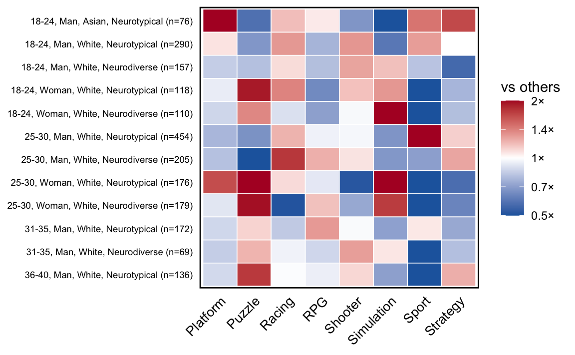
Figure 4 examines each demographic dimension in isolation, but players simultaneously occupy multiple demographic categories. Figure 5 presents a heatmap investigating potential intersectional trends using the same leave-one-out methodology as the radar charts, whereby each cell shows how an intersection’s genre proportion compares to everyone not in that intersection.
Results indicate that several of the genre trends observed in Figure 4 may be driven by intersectional trends. For example, the preference among women for puzzle games was particularly strong among 25–30 White woman, both neurodiverse and neurotypical, while the preference for strategy games was strongest in the 18-24 neurotypical Asian men group. Intersectional results should be interpreted with caution, due to the smaller sample sizes within each intersection and the inherent idiosyncrasies of the full sample.
The preceding analyses reveal differences in central tendency across demographic groups, but these visualizations can obscure how much of the total variation in play behavior lies between groups versus within groups. If between-group variance is small relative to within-group variance, demographic categories explain little of the overall heterogeneity in how people play—even if group means differ noticeably.
To quantify how much of the variation in play behavior is attributable to demographic categories versus individual differences, I calculated the proportion of total variance in an outcome that lies between groups rather than within groups, computed as SS_between / SS_total. For the combined estimate, I fit a multiple linear regression predicting each outcome from all four demographic variables simultaneously (age group, gender, ethnicity, and neurodiversity) and extracted \(R^2\), which represents the total variance explained by the full demographic profile. Values near zero indicate that demographic categories explain little of the overall heterogeneity in play behavior, even when group means differ noticeably.
# Function to calculate eta-squared (proportion of variance between groups)
calc_eta_sq <- function(outcome, grouping) {
  data <- tibble(y = outcome, g = grouping) |>
    filter(!is.na(y), !is.na(g))

  if (nrow(data) < 10 || n_distinct(data$g) < 2) {
    return(NA_real_)
  }

  grand_mean <- mean(data$y)
  group_stats <- data |>
    group_by(g) |>
    summarise(m = mean(y), n = n(), .groups = "drop")

  ss_between <- sum(group_stats$n * (group_stats$m - grand_mean)^2)
  ss_total <- sum((data$y - grand_mean)^2)

  if (ss_total == 0) {
    return(NA_real_)
  }
  ss_between / ss_total
}

# Calculate genre diversity (Shannon entropy) per person
genre_diversity <- genre_playtime_primary |>
  group_by(pid, genre_clean) |>
  summarise(minutes = sum(minutes, na.rm = TRUE), .groups = "drop") |>
  group_by(pid) |>
  mutate(prop = minutes / sum(minutes)) |>
  summarise(
    genre_entropy = -sum(prop * log(prop + 1e-10)),
    n_genres = n_distinct(genre_clean),
    .groups = "drop"
  )

# Build person-level dataset with all outcomes
# Note: person_data already contains is_neurotypical, is_adhd, is_autism from demographics join
variance_data <- person_data |>
  left_join(
    person_sessions |> select(pid, n_sessions, median_duration),
    by = "pid"
  ) |>
  left_join(
    person_temporal |> select(pid, top3_share, weekend_prop),
    by = "pid"
  ) |>
  left_join(genre_diversity, by = "pid") |>
  mutate(
    neuro_simple = case_when(
      is_neurotypical ~ "Neurotypical",
      is_adhd | is_autism ~ "Neurodiverse",
      TRUE ~ NA_character_
    )
  )

# Define outcomes with labels and categories
outcomes <- tribble(
  ~var              , ~label                  , ~category     ,
  "weekly_hours"    , "Weekly hours"          , "Volume"      ,
  "n_sessions"      , "Session count"         , "Volume"      ,
  "median_duration" , "Session duration"      , "Volume"      ,
  "genre_entropy"   , "Genre diversity"       , "Composition" ,
  "n_genres"        , "Genres played"         , "Composition" ,
  "top3_share"      , "Routine concentration" , "Temporal"    ,
  "weekend_prop"    , "Weekend concentration" , "Temporal"
)

# Define demographics (neuro_simple collapses non-exclusive neuro categories)
demo_vars <- c("age_group", "gender", "ethnicity", "neuro_simple")
demo_labels <- c("Age", "Gender", "Ethnicity", "Neurodiversity")

# Calculate eta-squared for each outcome × demographic combination
eta_results <- map_dfr(seq_len(nrow(outcomes)), function(i) {
  outcome_var <- outcomes$var[i]
  outcome_label <- outcomes$label[i]
  outcome_category <- outcomes$category[i]

  map_dfr(seq_along(demo_vars), function(j) {
    demo_var <- demo_vars[j]
    demo_label <- demo_labels[j]

    eta_sq <- calc_eta_sq(
      variance_data[[outcome_var]],
      variance_data[[demo_var]]
    )

    tibble(
      outcome = outcome_label,
      category = outcome_category,
      demographic = demo_label,
      eta_sq = eta_sq
    )
  })
}) |>
  filter(!is.na(eta_sq))

# Calculate combined R² (all demographics in one model) for each outcome
calc_combined_r2 <- function(data, outcome_var, demo_vars) {
  # Build formula with all demographic predictors
  formula_str <- glue("{outcome_var} ~ {paste(demo_vars, collapse = ' + ')}")

  # Filter to complete cases
  model_data <- data |>
    select(all_of(c(outcome_var, demo_vars))) |>
    filter(if_all(everything(), ~ !is.na(.)))

  if (nrow(model_data) < 10) {
    return(NA_real_)
  }

  # Fit linear model and extract R²
  fit <- lm(as.formula(formula_str), data = model_data)
  summary(fit)$r.squared
}

combined_results <- map_dfr(seq_len(nrow(outcomes)), function(i) {
  outcome_var <- outcomes$var[i]
  outcome_label <- outcomes$label[i]
  outcome_category <- outcomes$category[i]

  r2 <- calc_combined_r2(variance_data, outcome_var, demo_vars)

  tibble(
    outcome = outcome_label,
    category = outcome_category,
    demographic = "Combined",
    eta_sq = r2
  )
}) |>
  filter(!is.na(eta_sq))

# Merge individual and combined results
eta_results <- bind_rows(eta_results, combined_results)

# Robustness check: steelman model with splines on age + all two-way interactions
# Uses continuous age instead of age_group, natural splines (4 df), and all interactions
calc_steelman_r2 <- function(data, outcome_var) {
  model_data <- data |>
    select(all_of(c(outcome_var, "age", "gender", "ethnicity", "neuro_simple"))) |>
    filter(if_all(everything(), ~ !is.na(.)))

  if (nrow(model_data) < 50) return(NA_real_)

  # Formula with splines on age and all two-way interactions
  fit <- lm(
    as.formula(glue(
      "{outcome_var} ~ splines::ns(age, df = 4) * gender + splines::ns(age, df = 4) * ethnicity +
       splines::ns(age, df = 4) * neuro_simple + gender * ethnicity +
       gender * neuro_simple + ethnicity * neuro_simple"
    )),
    data = model_data
  )
  summary(fit)$r.squared
}

steelman_results <- map_dfr(seq_len(nrow(outcomes)), function(i) {
  tibble(
    outcome = outcomes$label[i],
    steelman_r2 = calc_steelman_r2(variance_data, outcomes$var[i])
  )
}) |>
  filter(!is.na(steelman_r2))

# Inline variable for maximum steelman R²
max_steelman_r2 <- max(steelman_results$steelman_r2, na.rm = TRUE)
max_steelman_r2_pct <- round(100 * max_steelman_r2, 1)

# Format steelman results for joining
steelman_fmt <- steelman_results |>
  mutate(
    `Combined (full)` = scales::percent(steelman_r2, accuracy = 0.1) |>
      str_replace("%", "\\\\%")
  ) |>
  select(outcome, `Combined (full)`)

# Pivot to wide format for table display
eta_wide <- eta_results |>
  mutate(
    eta_pct = scales::percent(eta_sq, accuracy = 0.1) |>
      str_replace("%", "\\\\%")
  ) |>
  select(category, outcome, demographic, eta_pct) |>
  pivot_wider(
    names_from = demographic,
    values_from = eta_pct
  ) |>
  rename(`Combined (main effects)` = Combined) |>
  left_join(steelman_fmt, by = "outcome") |>
  arrange(
    factor(category, levels = c("Volume", "Composition", "Temporal")),
    outcome
  )

# Build table with category header rows
eta_table <- bind_rows(
  tibble(
    Outcome = "Volume",
    Age = "",
    Gender = "",
    Ethnicity = "",
    Neuro = "",
    `Combined (main effects)` = "",
    `Combined (full)` = ""
  ),
  eta_wide |>
    filter(category == "Volume") |>
    select(Outcome = outcome, Age, Gender, Ethnicity, Neuro = Neurodiversity, `Combined (main effects)`, `Combined (full)`),
  tibble(
    Outcome = "Composition",
    Age = "",
    Gender = "",
    Ethnicity = "",
    Neuro = "",
    `Combined (main effects)` = "",
    `Combined (full)` = ""
  ),
  eta_wide |>
    filter(category == "Composition") |>
    select(Outcome = outcome, Age, Gender, Ethnicity, Neuro = Neurodiversity, `Combined (main effects)`, `Combined (full)`),
  tibble(
    Outcome = "Temporal",
    Age = "",
    Gender = "",
    Ethnicity = "",
    Neuro = "",
    `Combined (main effects)` = "",
    `Combined (full)` = ""
  ),
  eta_wide |>
    filter(category == "Temporal") |>
    select(Outcome = outcome, Age, Gender, Ethnicity, Neuro = Neurodiversity, `Combined (main effects)`, `Combined (full)`)
)

# Identify header rows for styling (rows where Age is empty = category headers)
header_rows <- which(eta_table$Age == "")

eta_table |>
  tt(
    notes = "Combined (main effects) = R² from multiple regression with separate, linear and simultaneous demographic predictors. Combined (full) = R² with splines on age and all two-way interactions. Neuro = Neurodiversity (Neurotypical vs. ADHD/autism)."
  ) |>
  style_tt(i = header_rows, bold = TRUE) |>
  style_tt(fontsize = 0.85) |>
  style_tt(i = 0, bold = TRUE)
# Inline variables for combined variance
max_combined_r2 <- combined_results |>
  summarise(max_r2 = max(eta_sq, na.rm = TRUE)) |>
  pull(max_r2)
max_combined_r2_pct <- round(100 * max_combined_r2, 1)

max_single_eta <- eta_results |>
  filter(demographic != "Combined") |>
  summarise(max_eta = max(eta_sq, na.rm = TRUE)) |>
  pull(max_eta)
max_single_eta_pct <- round(100 * max_single_eta, 1)| Outcome | Age | Gender | Ethnicity | Neuro | Combined (main effects) | Combined (full) |
|---|---|---|---|---|---|---|
| Combined (main effects) = R² from multiple regression with separate, linear and simultaneous demographic predictors. Combined (full) = R² with splines on age and all two-way interactions. Neuro = Neurodiversity (Neurotypical vs. ADHD/autism). | ||||||
| Volume | ||||||
| Session count | 0.6\% | 2.5\% | 0.4\% | 0.0\% | 3.2\% | 5.4\% |
| Session duration | 0.5\% | 0.0\% | 0.3\% | 0.0\% | 0.9\% | 4.6\% |
| Weekly hours | 0.1\% | 2.7\% | 0.3\% | 0.2\% | 3.5\% | 5.0\% |
| Composition | ||||||
| Genre diversity | 0.2\% | 0.8\% | 0.5\% | 0.6\% | 2.2\% | 3.4\% |
| Genres played | 0.4\% | 1.2\% | 0.6\% | 1.1\% | 3.3\% | 4.8\% |
| Temporal | ||||||
| Routine concentration | 0.8\% | 0.5\% | 0.7\% | 1.1\% | 3.2\% | 5.1\% |
| Weekend concentration | 0.7\% | 0.1\% | 0.0\% | 0.1\% | 0.8\% | 2.5\% |
# Calculate per-person proportion of playtime in shooter games
person_shooter_prop <- genre_playtime_primary |>
  group_by(pid, gender) |>
  summarise(
    prop_shooter = sum(minutes[genre_clean == "Shooter"], na.rm = TRUE) /
      sum(minutes),
    .groups = "drop"
  )

# Aggregate proportion of shooter playtime by gender (weighted by playtime)
gender_shooter_props <- genre_playtime_primary |>
  filter(gender %in% c("Man", "Woman")) |>
  group_by(gender) |>
  summarise(
    prop_shooter = sum(minutes[genre_clean == "Shooter"], na.rm = TRUE) /
      sum(minutes),
    .groups = "drop"
  )

men_avg_shooter <- gender_shooter_props |>
  filter(gender == "Man") |>
  pull(prop_shooter)
women_avg_shooter <- gender_shooter_props |>
  filter(gender == "Woman") |>
  pull(prop_shooter)

# Women who exceed the men's average
women_above_men <- person_shooter_prop |>
  filter(gender == "Woman", prop_shooter > men_avg_shooter)

# Summary stats
n_women_total <- person_shooter_prop |> filter(gender == "Woman") |> nrow()
n_women_above <- nrow(women_above_men)
pct_women_above <- round(100 * n_women_above / n_women_total, 1)

# Results for inline use
men_shooter_pct <- round(100 * men_avg_shooter, 1)
women_shooter_pct <- round(100 * women_avg_shooter, 1)
women_above_result <- glue("{n_women_above} ({pct_women_above}%)")
Results in Table 2 show that across all outcomes and demographic dimensions, the vast majority of variance in play behavior is within-group rather than between-group. Demographic categories explain less than 3% of total variance in every case, with most values below 1%. Even in a more parameterized specification with flexible age effects and all two-way interactions, the maximum variance explained was 5.4%.
In short, individuals within the same demographic group differ from one another far more than group averages differ from each other. This pattern holds across volume, composition, and temporal outcomes, reinforcing that demographic labels capture only a small slice of the heterogeneity in how people play.
The results presented here show a variety of trends among demographic groups in a diverse sample of UK and US adult video game players. Many these have been documented in prior survey-based research, such as the prevalence of sports game play among men and simulation game play among women (Phan et al., 2012) or the preference for RPGs among adults with autism (Mazurek et al., 2015). Other patterns are intuitive and have been theorized, but rarely directly observed and quantified in naturalistic behavioral data, such as the 1 hour earlier peak time and higher weekend concentration for older players (Ream et al., 2013).
However, despite the presence of these trends, the overall picture is one of substantial heterogeneity within groups, and thus overlap between them. For every observed difference, there are many individuals in the “opposite” group who show the same behavior. For example, although there is a marked difference in the average proportion of time men and women in the sample spent playing games in the shooter genre (33% vs 24.4% on average), there are still 208 (17%) women who have a higher shooter proportion than the average man. Results showing that effectively all permutations of play volume, timing and genre allocation are present in all demographic groups serves as a form of counter-stereotypical examples, a method recommended for reducing and reversing implicit biases in games culture (Flanagan & Kaufman, 2017).
In other words: while trends emerge at a bird’s eye view, knowing an individual’s complete demographic profile tells us remarkably little about their actual play behavior. Even with all demographic variables combined, a researcher could explain at most 5.4% of the variance in any single play outcome (Table 2). These findings echo early trace data studies showing demographic categories explain minimal variance in play patterns (Williams et al., 2008), but extend them to contemporary multi-platform contexts and provide explicit variance decomposition.
It is vital to interpret these results with care, and to avoid overgeneralization or stereotyping. The observed differences do not necessarily reflect stable preferences or inherent traits of demographic groups, but rather patterns of behavior that emerge from a complex interplay of structural factors, cultural contexts, and individual circumstances. For example, differences in temporal play patterns may reflect differences in work schedules (e.g., Lee & Chen, 2023), caregiving responsibilities (e.g., Wang et al., 2018), accessibility concerns (Porter & Kientz, 2013), or availability of gaming platforms (e.g., Ha & Kim, 2024), rather than intrinsic preferences for when to play. Similarly, genre preferences may be shaped by factors such as marketing, social norms, or peer influence, rather than inherent tastes. For example, it is long-established that White adult male characters are over-represented among video game characters, while Black female characters and many other groups are under-represented (Jones et al., 2025; Williams, Martins, et al., 2009; cf. Gardner & Tanenbaum, 2018), which may contribute to the observed differences in genre allocation.
With those caveats in mind, this work still offers several contributions for the field: it offers a foundation for hypothesis generation, theory specification, and study design; highlights behavioral dimensions such as routine concentration or genre diversity that may be more informative outcomes than total playtime; and points to the value of behavioral trace data in revealing how people actually play, rather than what they say about their play.
These findings complicate how demographic categories should function in games HCI theory. When within-group variance is at least 18x larger than between-group variance, demographics may be valuable as contextual background variables but are unlikely to be useful as primary predictors of behavioral outcomes. Such empirical backing reinforces known challenges for theory, quantitative methods, and design.
On the theory side, I argue for improved specification of the specific mechanisms through which demographics matter rather than treating them as proxies for preferences. Although there is widespread recognition of the pitfalls of demographic essentialism at the theory level, empirical studies often use and interpret demographics are key predictors of outcomes such as motivational styles or player types (Yee, 2006), esports participation (Kordyaka et al., 2023), or internet gaming disorder (Lopez-Fernandez et al., 2019). Such use of demographic variables may serve as a proxy for preferences or behaviors, masking the underlying mechanistic differences on which the field could actually intervene. Future work with representative samples and/or qualitative methods can help unpack which of these trends generalize to other metrics of real-world play, and why they occur (access? cultural exposure? time constraints?).
Eventually, such work may allow mechanism-related variables to supplement demographics themselves in quantitative studies. Results here show that the use of demographics variables in statistical models should be carefully considered. Researchers should report and be mindful of effect sizes, and ensure that statistical significance of a particular demographic variable is not conflated with the practical significance thereof (Kirk, 1996; Vornhagen et al., 2020).
With regard to design, these results suggest that demographic categories may be useful for coarse segmentation, but heterogeneity will often be too large to reliably base more granular decisions such as design for diverse groups such as women or older players (Gerling et al., 2012; Kaufman et al., 2019). Behavioral segmentation based on characteristics like genre allocation and temporal play patterns, a well-established industry practice (Norman, 2020; Yin et al., 2025), offers a valuable alternative for many design or intervention decisions.
To reiterate, low predictive strength does not mean demographics have no value for design or analytics. Observed differences in temporal organization and engagement span suggest that features such as session length expectations, save mechanics, or live-service timing may differentially fit players with distinct demographic constraints (Figure 3). Similarly, genre portfolio patterns can inform decisions about cross-promotion, onboarding pathways, and content diversification strategies.
As highlighted throughout this piece, these data do not provide strong evidence for generalizable differences between groups. I did not apply weighting or conduct hypothesis tests. Observed differences should not be interpreted as stable preferences or group traits, as these data cannot meaningfully distinguish access effects from preference effects.
The gameplay behavior observed here is wide but shallow - while the data captured individuals’ play across a wide variety of titles (mean: 19.6 distinct titles per player), it does not capture their behavior within particular games. To advance knowledge on various topics typically studied using self-reports or in lab settings, deep game-level is needed instead: for example, avatar selection data to study the Proteus Effect (Yee & Bailenson, 2007), performance data to study skill acquisition (Ratan et al., 2015), and communications and friends data to understand gender differences in social behavior (Wilhelm, 2018). Achieving such advances will require more widespread adoption of the full trace data collection toolkit, ranging from data donation (Es & Nguyen, 2025; which has already proven successful for behavioral research on social media, e.g., Yap et al., 2024), scraping-based methods (Ballou et al., 2024), and existing APIs (e.g., Vuorre et al., 2021; although see Davidson et al., 2023 for transparency issues associated with platform-provided APIs).
Further, while the quasi-representative sampling strategy underlying this data produced a sample more diverse than many comparable studies of video game trace data (e.g., Ballou et al., 2024; Larrieu et al., 2023), the sample here is not random or representative of either the general population or of all video game players. Such trade-offs are inherent: with the exception of extremely rare studies that have access to population data via platform owners (e.g., Zendle et al., 2023), collecting demographic data requires contacting individual participants who may elect not to join the study. Selection biases are thus present with regard to willingness to share data, sufficient gaming on included platforms, and participation in the survey platforms from which recruitment took place (Prolific, PureProfile).
I particularly draw attention to the exclusion of mobile gaming due to insufficient data granularity, as previous results have shown that the demographics of mobile players systematically differ from those of other gaming platforms (Entertainment Software Association, 2025; Gottfried & Sidoti, 2024). Similarly, the lack of Xbox data among UK participants means recorded behavior and game composition differs across countries ; to mitigate this, the analyses intentionally do not compare the US and UK, but group all participants. The combination of selection biases present in the study also likely contributed to some of the surprising characteristics of the sample, such as high self-reported rates of neurodiversity.
In short, more representative or targeted samples, deep game-level data, and qualitative follow-up are all needed to build on this work. Future research should aim to disentangle access effects from preference effects, assess the generalizability of these patterns, and further unpack the lived experiences underlying observed demographic differences.
This study used publicly available behavioral trace data from Steam, Xbox, and Nintendo Switch to describe how play patterns vary across age, gender, ethnicity, and neurodiversity in a diverse sample of 3,768 US and UK adults. Results revealed a range of demographic differences in play volume, temporal organization, engagement span, and genre composition, many of which corroborate prior survey-based findings, while others (such as the earlier peak playtime among older players or the longer engagement spans among women and Black players) have rarely been directly observed in naturalistic data.
Yet the overarching finding is one of within-group heterogeneity: demographic characteristics collectively explained less than 6% of the variance in any dimension of play behavior examined. These results suggest that while demographic categories remain useful for coarse description and hypothesis generation, they are poor proxies for how any individual actually plays. Future work should aim to move beyond demographics as default predictors, instead investigating the structural, cultural, and individual-level mechanisms that give rise to the patterns observed here, and doing so with representative samples, deep game-level data, and methods that center players’ own accounts of their play.
[Redacted for anonymous peer review]
[Redacted for anonymous peer review]
A portion of the data in this study (Xbox and Nintendo Switch trace data) was collected via data-sharing agreements with Microsoft, Nintendo of America, and Nintendo of Europe. Industry partners did not contribute funding for the research or any of the researchers involved in conducting it, and had no role in the design, analysis, or publication of results.
The author declares no other potential financial, intellectual, or institutional conflicts of interests.
Claude Code (claude-opus-4-5-20251101) was used to prepare and document analysis code. The author takes full responsibility for the content of the analyses and any errors that may be present.
[Redacted]
tibble(
  Platform = c(
    "Nintendo",
    "Xbox (US only)",
    "Steam",
    "iOS",
    "Android"
  ),
  Source = c(
    "Nintendo of America/Europe data-sharing",
    "Microsoft data-sharing",
    "Custom web app (Gameplay.Science)",
    "iOS Screen Time screenshots",
    "Digital Wellbeing screenshots"
  ),
  `Account Linking` = c(
    "Participants share QR code identifier from Nintendo web interface; Nintendo retrieves and shares gameplay data",
    "Participants opt in via Xbox Insiders; Microsoft shares pseudonymized data",
    "Participants authenticate via Steam API (OpenID); gameplay monitored for study duration",
    "Screenshots of up to 3 weeks of gaming; data extracted via OCR",
    "Screenshots of up to 3 weeks of gaming; data extracted via OCR"
  ),
  `Data Type` = c(
    "Session records (game, time, duration) for first-party Nintendo games only",
    "Session records with anonymized titles; genre and age rating preserved",
    "Hourly aggregates per game.",
    "Daily aggregates",
    "Daily aggregates"
  )
) |>
  tt(
    notes = "Nintendo-published games accounted for 63 percent of Switch playtime in the sample.",
    width = 1
  ) |>
  style_tt(fontsize = 0.7) |>
style_tt(i = 0, bold = TRUE, align = "c")| Platform | Source | Account Linking | Data Type |
|---|---|---|---|
| Nintendo-published games accounted for 63 percent of Switch playtime in the sample. | |||
| Nintendo | Nintendo of America/Europe data-sharing | Participants share QR code identifier from Nintendo web interface; Nintendo retrieves and shares gameplay data | Session records (game, time, duration) for first-party Nintendo games only |
| Xbox (US only) | Microsoft data-sharing | Participants opt in via Xbox Insiders; Microsoft shares pseudonymized data | Session records with anonymized titles; genre and age rating preserved |
| Steam | Custom web app (Gameplay.Science) | Participants authenticate via Steam API (OpenID); gameplay monitored for study duration | Hourly aggregates per game. |
| iOS | iOS Screen Time screenshots | Screenshots of up to 3 weeks of gaming; data extracted via OCR | Daily aggregates |
| Android | Digital Wellbeing screenshots | Screenshots of up to 3 weeks of gaming; data extracted via OCR | Daily aggregates |
# Get top games per demographic group (excluding Xbox)
# First prepare data with neurodiversity as a single column
telemetry_with_demo <- hourly_telemetry |>
  filter(platform != "Xbox") |>
  left_join(demographics, by = "pid") |>
  filter(!is.na(age_group))

# Standard demographics (age, gender, ethnicity)
top_games_standard <- telemetry_with_demo |>
  pivot_longer(
    cols = c(age_group, gender, ethnicity),
    names_to = "demo_type",
    values_to = "demo_group"
  ) |>
  filter(!is.na(demo_group)) |>
  group_by(demo_type, demo_group, title_id) |>
  summarise(total_hours = sum(minutes, na.rm = TRUE) / 60, .groups = "drop")

# Neurodiversity (non-exclusive categories handled separately)
top_games_neuro <- bind_rows(
  telemetry_with_demo |>
    filter(is_neurotypical == TRUE) |>
    group_by(title_id) |>
    summarise(total_hours = sum(minutes, na.rm = TRUE) / 60, .groups = "drop") |>
    mutate(demo_type = "neurodiversity", demo_group = "Neurotypical"),
  telemetry_with_demo |>
    filter(is_adhd == TRUE) |>
    group_by(title_id) |>
    summarise(total_hours = sum(minutes, na.rm = TRUE) / 60, .groups = "drop") |>
    mutate(demo_type = "neurodiversity", demo_group = "ADHD"),
  telemetry_with_demo |>
    filter(is_autism == TRUE) |>
    group_by(title_id) |>
    summarise(total_hours = sum(minutes, na.rm = TRUE) / 60, .groups = "drop") |>
    mutate(demo_type = "neurodiversity", demo_group = "Autism spectrum")
)

top_games_by_demo <- bind_rows(top_games_standard, top_games_neuro) |>
  # Get top 5 per demographic group
  group_by(demo_type, demo_group) |>
  slice_max(total_hours, n = 5) |>
  mutate(rank = row_number()) |>
  ungroup() |>
  # Clean up demo_type names
  mutate(
    demo_type = case_when(
      demo_type == "age_group" ~ "Age",
      demo_type == "gender" ~ "Gender",
      demo_type == "ethnicity" ~ "Ethnicity",
      demo_type == "neurodiversity" ~ "Neurodiversity"
    )
  )

# Pivot to wide format for display
top_games_wide <- top_games_by_demo |>
  mutate(
    game_label = glue("{title_id}\n({scales::comma(round(total_hours))}h)")
  ) |>
  select(demo_type, demo_group, rank, game_label) |>
  pivot_wider(
    names_from = rank,
    values_from = game_label,
    names_prefix = "Rank "
  ) |>
  arrange(demo_type, demo_group) |>
  rename(Demographic = demo_type, Group = demo_group)

top_games_wide |>
  tt(width = 1) |>
  style_tt(fontsize = 0.6) |>
style_tt(i = 0, bold = TRUE)| Demographic | Group | Rank 1 | Rank 2 | Rank 3 | Rank 4 | Rank 5 |
|---|---|---|---|---|---|---|
| Age | 18-24 | Animal Crossing New Horizons (14,080h) | Marvel Rivals (10,507h) | The Legend of Zelda Tears of the Kingdom (8,281h) | Counter-Strike 2 (6,519h) | Splatoon 3 (6,194h) |
| Age | 25-30 | Animal Crossing New Horizons (16,075h) | Pokemon Scarlet / Violet (11,369h) | The Legend of Zelda Tears of the Kingdom (11,129h) | Marvel Rivals (8,187h) | Counter-Strike 2 (6,566h) |
| Age | 31-35 | The Legend of Zelda Tears of the Kingdom (5,047h) | Pokemon Scarlet / Violet (2,857h) | Animal Crossing New Horizons (2,814h) | FINAL FANTASY XIV Online (2,136h) | Football Manager 2024 (1,664h) |
| Age | 36-40 | The Legend of Zelda Tears of the Kingdom (3,128h) | Animal Crossing New Horizons (3,061h) | Pokemon Scarlet / Violet (2,870h) | Mario Kart 8 Deluxe (1,253h) | Football Manager 2024 (959h) |
| Ethnicity | Asian | Marvel Rivals (1,758h) | Umamusume: Pretty Derby (1,748h) | MapleStory (1,710h) | The Legend of Zelda Tears of the Kingdom (1,560h) | Pokemon Scarlet / Violet (1,508h) |
| Ethnicity | Black | Animal Crossing New Horizons (2,710h) | Marvel Rivals (2,047h) | Super Smash Bros Ultimate (1,697h) | Splatoon 3 (1,621h) | The Legend of Zelda Tears of the Kingdom (1,532h) |
| Ethnicity | Mixed/Multiple | Marvel Rivals (3,876h) | Animal Crossing New Horizons (2,723h) | FINAL FANTASY XIV Online (2,277h) | Pokemon Scarlet / Violet (1,918h) | The Legend of Zelda Tears of the Kingdom (1,660h) |
| Ethnicity | Other | Pokemon UNITE (1,399h) | Super Smash Bros Ultimate (1,069h) | Marvel Rivals (711h) | Umamusume: Pretty Derby (698h) | The Legend of Zelda Tears of the Kingdom (584h) |
| Ethnicity | White | Animal Crossing New Horizons (28,694h) | The Legend of Zelda Tears of the Kingdom (22,238h) | Pokemon Scarlet / Violet (16,978h) | Marvel Rivals (11,847h) | Counter-Strike 2 (10,766h) |
| Gender | Man | Pokemon Scarlet / Violet (13,868h) | The Legend of Zelda Tears of the Kingdom (13,449h) | Counter-Strike 2 (12,824h) | Marvel Rivals (12,164h) | Animal Crossing New Horizons (7,842h) |
| Gender | Non-binary/Other | Animal Crossing New Horizons (4,157h) | Baldur's Gate 3 (2,361h) | The Legend of Zelda Tears of the Kingdom (2,155h) | Warframe (1,973h) | Splatoon 3 (1,442h) |
| Gender | Woman | Animal Crossing New Horizons (23,987h) | The Legend of Zelda Tears of the Kingdom (11,980h) | Marvel Rivals (6,713h) | Pokemon Scarlet / Violet (6,417h) | Splatoon 3 (5,736h) |
| Neurodiversity | ADHD | Animal Crossing New Horizons (12,890h) | The Legend of Zelda Tears of the Kingdom (7,363h) | Marvel Rivals (6,823h) | Pokemon Scarlet / Violet (5,170h) | Baldur's Gate 3 (4,804h) |
| Neurodiversity | Autism spectrum | Animal Crossing New Horizons (8,301h) | The Legend of Zelda Tears of the Kingdom (6,134h) | Pokemon Scarlet / Violet (5,172h) | Splatoon 3 (4,536h) | Baldur's Gate 3 (4,077h) |
| Neurodiversity | Neurotypical | The Legend of Zelda Tears of the Kingdom (14,973h) | Animal Crossing New Horizons (14,348h) | Pokemon Scarlet / Violet (11,657h) | Marvel Rivals (10,916h) | Counter-Strike 2 (10,309h) |
# Use pre-calculated deviation (computed on all genres, then filtered for display)
build_radar_grid(
  genre_props_dev_plot_multi,
  group_ns_multi,
  top_genres,
  demo_colors,
  theme_radar,
  theme_radar_empty,
  theme_radar_label
)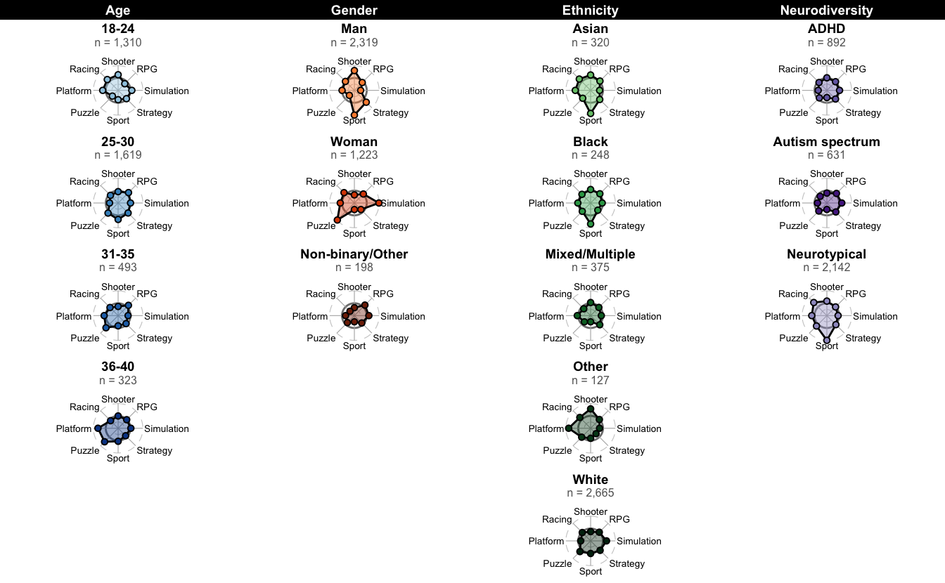
# Get all raw genres (before simplification)
games_all_genres <- games |>
  filter(!is.na(genres)) |>
  separate_rows(genres, sep = ",\\s*") |>
  distinct(original_name, genres) |>
  group_by(original_name) |>
  mutate(genre_weight = 1 / n()) |>

  ungroup()

# Calculate playtime by raw genre and demographic
genre_playtime_raw <- hourly_telemetry |>
  left_join(
    games_all_genres,
    by = c("title_id" = "original_name"),
    relationship = "many-to-many"
  ) |>
  filter(!is.na(genres)) |>
  mutate(minutes_weighted = minutes * genre_weight) |>
  left_join(demographics, by = "pid") |>
  filter(!is.na(age_group))

# Step 1: Calculate individual-level genre proportions
individual_genre_props <- genre_playtime_raw |>
  group_by(pid, genres) |>
  summarise(genre_minutes = sum(minutes_weighted, na.rm = TRUE), .groups = "drop") |>
  group_by(pid) |>
  mutate(individual_prop = genre_minutes / sum(genre_minutes) * 100) |>
  ungroup()

# Join demographic info back
individual_with_demo <- individual_genre_props |>
  left_join(
    demographics |> select(pid, age_group, gender, ethnicity, is_neurotypical, is_adhd, is_autism),
    by = "pid"
  )

# Helper to calculate median props for a grouping variable
calc_median_props <- function(data, group_var, demo_name) {
  data |>
    filter(!is.na(.data[[group_var]])) |>
    group_by(.data[[group_var]], genres) |>
    summarise(prop = median(individual_prop, na.rm = TRUE), .groups = "drop") |>
    rename(group = all_of(group_var)) |>
    mutate(demo = demo_name)
}

# Calculate for all demographics using median of individual allocations
all_genre_props <- bind_rows(
  calc_median_props(individual_with_demo, "age_group", "Age"),
  calc_median_props(individual_with_demo, "gender", "Gender"),
  calc_median_props(individual_with_demo, "ethnicity", "Ethnicity"),
  # Neurodiversity (non-exclusive categories)
  bind_rows(
    individual_with_demo |>
      filter(is_neurotypical == TRUE) |>
      group_by(genres) |>
      summarise(prop = median(individual_prop, na.rm = TRUE), .groups = "drop") |>
      mutate(group = "Neurotypical"),
    individual_with_demo |>
      filter(is_adhd == TRUE) |>
      group_by(genres) |>
      summarise(prop = median(individual_prop, na.rm = TRUE), .groups = "drop") |>
      mutate(group = "ADHD"),
    individual_with_demo |>
      filter(is_autism == TRUE) |>
      group_by(genres) |>
      summarise(prop = median(individual_prop, na.rm = TRUE), .groups = "drop") |>
      mutate(group = "Autism")
  ) |>
    mutate(demo = "Neuro")
) |>
  mutate(prop_fmt = sprintf("%.1f", prop))

# Create genre mapping - only show if it maps to one of the TOP 8 genres in radar
genre_mapping <- tibble(genres = unique(all_genre_props$genres)) |>
  mutate(
    cleaned = clean_genre(genres),
    abbreviated = abbreviate_genre(cleaned),
    # Only show mapping if it's in the top_genres used in radar
    maps_to = if_else(abbreviated %in% top_genres, abbreviated, "—")
  ) |>
  select(genres, maps_to)

# Calculate overall mean to sort by
genre_order <- all_genre_props |>
  group_by(genres) |>
  summarise(mean_prop = mean(prop), .groups = "drop") |>
  arrange(desc(mean_prop)) |>
  pull(genres)

# Pivot to wide format with readable column names (~5 chars)
genre_table <- all_genre_props |>
  mutate(
    group_abbr = case_when(
      group == "18-24" ~ "18-24",
      group == "25-30" ~ "25-30",
      group == "31-35" ~ "31-35",
      group == "36-40" ~ "36-40",
      group == "Man" ~ "Man",
      group == "Woman" ~ "Woman",
      group == "Non-binary/Other" ~ "NB/Ot",
      group == "Asian" ~ "Asian",
      group == "Black" ~ "Black",
      group == "Mixed/Multiple" ~ "Mixed",
      group == "Other" ~ "Other",
      group == "White" ~ "White",
      group == "Neurotypical" ~ "Neuro",
      group == "ADHD" ~ "ADHD",
      group == "Autism" ~ "Autis",
      TRUE ~ group
    )
  ) |>
  select(genres, group_abbr, prop_fmt) |>
  pivot_wider(
    names_from = group_abbr,
    values_from = prop_fmt,
    values_fill = "0.0"
  ) |>
  left_join(genre_mapping, by = "genres") |>
  mutate(
    genres = str_replace_all(genres, "&", "and"),
    genres = factor(genres, levels = str_replace_all(genre_order, "&", "and"))
  ) |>
  arrange(genres) |>
  select(Genre = genres, Radar = maps_to, everything())

genre_table |>
  tt(
    notes = "Values are median percentages of individual players' genre allocations (matching radar chart methodology). 'Radar' shows the simplified category used in the main text radar plot (— if genre is not included in the 8 simplified categories). Neuro = Neurotypical, Autis = Autism spectrum.",
    width = 1
  ) |>
  style_tt(fontsize = 0.5) |>
style_tt(i = 0, bold = TRUE, fontsize = 0.45)| Genre | Radar | 18-24 | 25-30 | 31-35 | 36-40 | Man | NB/Ot | Woman | Asian | Black | Mixed | Other | White | Neuro | ADHD | Autis |
|---|---|---|---|---|---|---|---|---|---|---|---|---|---|---|---|---|
| Values are median percentages of individual players' genre allocations (matching radar chart methodology). 'Radar' shows the simplified category used in the main text radar plot (— if genre is not included in the 8 simplified categories). Neuro = Neurotypical, Autis = Autism spectrum. | ||||||||||||||||
| Adventure | — | 14.8 | 17.3 | 20.0 | 20.3 | 16.5 | 15.7 | 18.1 | 17.4 | 16.4 | 15.1 | 14.3 | 17.5 | 17.5 | 15.2 | 16.4 |
| Role-playing (RPG) | RPG | 11.1 | 14.5 | 15.4 | 14.0 | 12.7 | 15.0 | 13.1 | 13.2 | 13.5 | 12.5 | 13.6 | 13.1 | 13.1 | 13.3 | 14.4 |
| Shooter | Shooter | 15.3 | 12.5 | 9.9 | 13.4 | 14.4 | 8.7 | 9.5 | 16.0 | 14.6 | 14.2 | 20.0 | 12.2 | 13.9 | 13.0 | 11.0 |
| Simulator | Simulation | 11.4 | 10.7 | 8.5 | 11.1 | 8.3 | 12.2 | 17.2 | 8.6 | 10.4 | 9.6 | 7.5 | 11.3 | 10.4 | 10.7 | 12.3 |
| Indie | — | 9.9 | 10.0 | 9.3 | 10.6 | 9.1 | 12.4 | 12.0 | 10.5 | 8.6 | 11.0 | 6.9 | 9.9 | 9.3 | 10.0 | 10.1 |
| Strategy | Strategy | 6.2 | 8.0 | 7.4 | 6.5 | 7.3 | 5.4 | 7.2 | 6.4 | 5.4 | 7.8 | 4.2 | 7.4 | 7.3 | 6.5 | 7.7 |
| Platform | Platform | 3.2 | 2.4 | 3.3 | 4.5 | 2.8 | 1.7 | 3.3 | 3.2 | 3.1 | 2.6 | 4.2 | 2.7 | 3.1 | 2.1 | 2.2 |
| Sport | Sport | 2.0 | 2.9 | 2.2 | 2.7 | 3.0 | 1.0 | 1.5 | 4.4 | 4.4 | 1.2 | 2.2 | 2.4 | 3.2 | 1.6 | 1.4 |
| Puzzle | Puzzle | 1.9 | 2.1 | 2.9 | 3.8 | 1.8 | 1.8 | 3.6 | 1.6 | 1.8 | 1.5 | 3.2 | 2.3 | 2.5 | 1.8 | 2.0 |
| Tactical | Strategy | 3.1 | 2.4 | 2.4 | 2.2 | 3.1 | 0.9 | 1.7 | 3.3 | 1.6 | 1.6 | 1.7 | 2.8 | 3.1 | 2.0 | 2.2 |
| Racing | Racing | 2.5 | 1.9 | 1.8 | 1.9 | 2.0 | 0.9 | 2.4 | 2.9 | 2.3 | 1.7 | 2.8 | 2.1 | 2.6 | 1.8 | 1.7 |
| Turn-based strategy (TBS) | Strategy | 1.7 | 2.0 | 2.2 | 3.2 | 1.9 | 1.7 | 2.2 | 2.9 | 2.1 | 1.2 | 1.9 | 2.0 | 2.2 | 1.7 | 1.9 |
| Real Time Strategy (RTS) | Strategy | 1.2 | 2.4 | 1.8 | 2.3 | 2.1 | 1.8 | 1.3 | 2.8 | 1.2 | 2.2 | 2.7 | 1.7 | 2.3 | 1.4 | 1.7 |
| Card and Board Game | Puzzle | 1.2 | 1.9 | 2.3 | 2.6 | 1.3 | 1.0 | 3.2 | 2.4 | 1.9 | 1.7 | 1.4 | 1.6 | 2.2 | 1.3 | 1.3 |
| Arcade | — | 2.0 | 1.3 | 1.4 | 1.6 | 1.4 | 0.9 | 2.1 | 2.3 | 2.5 | 1.1 | 3.3 | 1.5 | 1.7 | 1.3 | 1.4 |
| Hack and slash/Beat 'em up | — | 1.2 | 1.5 | 1.5 | 1.3 | 1.5 | 1.2 | 1.0 | 2.4 | 1.3 | 1.6 | 1.5 | 1.3 | 1.5 | 1.0 | 1.2 |
| Visual Novel | — | 1.0 | 0.9 | 1.4 | 1.3 | 0.8 | 1.5 | 1.2 | 1.8 | 2.7 | 1.2 | 1.4 | 0.7 | 1.1 | 0.9 | 0.8 |
| Fighting | — | 1.0 | 0.8 | 0.9 | 1.1 | 1.1 | 0.6 | 0.7 | 1.3 | 1.9 | 1.5 | 1.5 | 0.8 | 1.0 | 0.8 | 0.6 |
| MOBA | Strategy | 0.7 | 1.2 | 2.1 | 0.9 | 1.1 | 0.5 | 0.8 | 0.7 | 0.8 | 0.7 | 1.1 | 1.1 | 1.0 | 1.2 | 0.8 |
| Music | — | 0.7 | 0.5 | 1.0 | 1.0 | 0.5 | 1.0 | 0.7 | 1.4 | 0.6 | 0.6 | 0.3 | 0.5 | 0.5 | 0.7 | 0.8 |
| Point-and-click | — | 0.4 | 0.5 | 0.7 | 0.4 | 0.3 | 0.7 | 0.7 | 0.2 | 3.0 | 0.7 | 0.1 | 0.5 | 0.5 | 0.4 | 0.5 |
| Quiz/Trivia | Puzzle | 0.2 | 0.1 | 0.3 | 0.7 | 0.2 | 0.4 | 0.1 | 0.1 | 0.2 | 0.1 | 0.1 | 0.2 | 0.2 | 0.2 | 0.4 |
| Pinball | — | 0.2 | 0.1 | 0.4 | 0.0 | 0.2 | 0.0 | 0.0 | 0.0 | 0.9 | 0.0 | 0.2 | 0.1 | 0.2 | 0.0 | 0.1 |