---
title: |
All BANG, little buck: Need-related experiences are weakly linked with behavior in the video game domain
author:
- name: Nick Ballou
corresponding: true
orcid: 0000-0003-4126-0696
email: nick@nickballou.com
affiliations:
- ref: 1
- ref: 2
roles:
- conceptualization
- data curation
- investigation
- methodology
- formal analysis
- visualization
- writing
- editing
- name: Tamás Andrei Földes
corresponding: false
orcid: 0000-0002-0623-9149
email: tamas.foldes@oii.ox.ac.uk
affiliations:
- ref: 2
roles:
- data curation
- methodology
- validation
- editing
- name: Matti Vuorre
corresponding: false
orcid: 0000-0001-5052-066X
email: mjvuorre@uvt.nl
affiliations:
- ref: 3
roles:
- methodology
- funding acquisition
- editing
- name: Thomas Hakman
corresponding: false
orcid: 0009-0009-8292-2482
email: thomas.hakman@oii.ox.ac.uk
affiliations:
- ref: 2
roles:
- investigation
- data curation
- editing
- name: Kristoffer Magnusson
corresponding: false
orcid: 0000-0003-0713-0556
affiliations:
- ref: 4
- ref: 2
roles:
- software
- editing
- name: Andrew K Przybylski
corresponding: true
email: andy.przybylski@oii.ox.ac.uk
orcid: 0000-0001-5547-2185
affiliations:
- ref: 2
roles:
- conceptualization
- funding acquisition
- project administration
- editing
affiliations:
- id: 1
name: Imperial College London
department: Dyson School of Design Engineering
- id: 2
name: University of Oxford
department: Oxford Internet Institute
- id: 3
name: Tilburg University
department: Department of Social Psychology
- id: 4
name: Karolinska Institute
csl: https://www.zotero.org/styles/apa
bibliography: references.bib
keywords: [motivation, digital trace data, video games, self-determination theory, displacement, compensatory behavior]
editor_options:
chunk_output_type: console
markdown:
wrap: none
knitr:
opts_chunk:
cache: true
warning: false
message: false
fig-width: 6
fig-asp: 0.618
out-width: 80%
fig-align: center
code-links: repo
format:
html:
theme:
light: united
dark: darkly
toc: true
toc-depth: 2
toc-location: right
number-sections: true
fontsize: 13pt
code-fold: true
code-summary: "Show code"
code-tools: true
echo: true
embed-resources: false
page-layout: article
grid:
body-width: 900px
margin-width: 250px
other-links:
- text: Stage 1 Registered Report
href: https://osf.io/pb5nu
icon: file-pdf
- text: Data
href: https://zenodo.org/records/17609160
icon: link
preprint-typst:
echo: false
wordcount: true
theme: jou
citeproc: true
mainfont: "Liberation Serif"
sansfont: "Liberation Sans"
include-before-body:
- text: "#show <refs>: set par(hanging-indent: 1.4em)"
docx:
echo: false
---
```{r}
#| label: libraries
#| code-summary: "Show code (Load required R packages)"
#| cache: false
library(tidyverse)
library(glue)
library(glmmTMB)
library(lme4)
library(marginaleffects)
library(mice)
library(howManyImputations)
library(future)
library(modelsummary)
library(lubridate)
library(DHARMa)
library(brms)
library(broom.mixed)
library(psych)
library(tinytable)
library(litedown)
library(patchwork)
library(ggridges)
library(ggdist)
library(splines)
library(scales)
library(janitor)
```
```{r}
#| label: setup
#| code-summary: "Show code (Set random seed and global options)"
#| cache: false
set.seed(8675309)
options(scipen = 999, timeout = 600)

theme_set(theme_minimal())
theme_update(
  plot.background = element_rect(fill = "white", color = NA),
  panel.background = element_rect(fill = "white", color = NA),
  strip.background = element_rect(fill = "black"),
  strip.text = element_text(color = "white", size = 10),
  axis.text.y = element_text(color = "black", size = 10),
  axis.text.x = element_text(color = "black", size = 10),
  panel.grid.minor = element_blank(),
  panel.border = element_rect(
    colour = "black",
    fill = NA,
    linewidth = 1
  )
)

# Define consistent color palette for all visualizations
colors <- list(
  game_ns = "#009988", # Teal for game need satisfaction
  global_ns = "#44BB99", # Light teal for global need satisfaction
  global_nf = "#EE6677", # Red for global need frustration
  nintendo = "#E60012", # Nintendo red
  xbox = "#107C10", # Xbox green
  steam = "#215e8a", # Steam dark blue
  within = "#228833", # Green for within-person variance
  between = "#BBBBBB" # Gray for between-person variance
)

# Define human-readable labels for snake_case column names
labels <- c(
  # Base variables
  "game_ns" = "Game need satisfaction",
  "game_nf" = "Game need frustration",
  "global_ns" = "Global need satisfaction",
  "global_nf" = "Global need frustration",
  "session_length" = "Session length",
  "session_gap" = "Time to next session",
  # Within-person
  "game_ns_cw" = "Game need satisfaction (within)",
  "game_nf_cw" = "Game need frustration (within)",
  "global_ns_cw" = "Global need satisfaction (within)",
  "global_nf_cw" = "Global need frustration (within)",
  # Between-person
  "game_ns_cb" = "Game need satisfaction (between)",
  "game_nf_cb" = "Game need frustration (between)",
  "global_ns_cb" = "Global need satisfaction (between)",
  "global_nf_cb" = "Global need frustration (between)",
  # Within-person (alternate)
  "game_ns (within-person)" = "Game need satisfaction (within-person)",
  "global_ns (within-person)" = "Global need satisfaction (within-person)",
  "global_nf (within-person)" = "Global need frustration (within-person)",
  # Between-person (alternate)
  "game_ns (between-person)" = "Game need satisfaction (between-person)",
  "global_ns (between-person)" = "Global need satisfaction (between-person)",
  "global_nf (between-person)" = "Global need frustration (between-person)",
  # Interaction
  "game_ns_cw:global_nf_cw" = "Game need satisfaction × Global need frustration (within)",
  # Displacement
  "displaced_core_domain" = "Displaced core domain",
  "displaced_core_domainTRUE" = "Displaced core domain",
  # Variance components
  "Within-person" = "Within-person",
  "Between-person" = "Between-person",
  # Other
  "(Intercept)" = "Intercept"
)

# Load custom functions
source("R/helpers.R")
```
```{r}
#| label: load-data
#| code-summary: "Show code (Download and load raw data from Zenodo)"
# Download data from Zenodo (one-time download, then cached locally)
zenodo_url <- "https://zenodo.org/records/17609160/files/digital-wellbeing/open-play-v1.0.0.zip?download=1"
zip_path <- "data/open-play-v1.0.0.zip"

if (!file.exists(zip_path)) {
  dir.create(dirname(zip_path), showWarnings = FALSE, recursive = TRUE)

  # Set longer timeout for large file (194MB) - default is 60 seconds
  options(timeout = max(600, getOption("timeout")))

  message("Downloading 194MB file from Zenodo (may take a few minutes)...")
  tryCatch(
    {
      download.file(zenodo_url, zip_path, mode = "wb", method = "libcurl")
      message("Download complete!")
    },
    error = function(e) {
      message("Download failed. Please download manually from:")
      message(zenodo_url)
      message(glue("And save to: {normalizePath(zip_path, mustWork = FALSE)}"))
      stop(e)
    }
  )
}

# Extract zip if not already extracted
extract_dir <- "data/open-play-v1.0.0"
if (!dir.exists(extract_dir)) {
  message("Extracting zip archive...")
  unzip(zip_path, exdir = "data")
  # Rename the extracted folder to a simpler name
  extracted_folder <- list.dirs("data", recursive = FALSE, full.names = TRUE)
  extracted_folder <- extracted_folder[grepl(
    "digital-wellbeing-open-play",
    extracted_folder
  )]
  if (length(extracted_folder) == 1 && extracted_folder != extract_dir) {
    file.rename(extracted_folder, extract_dir)
  }
}

# Read files from extracted directory
intake <- read_csv(
  file.path(extract_dir, "data/clean/survey_intake.csv.gz"),
  guess_max = 10000
)
surveys <- read_csv(file.path(
  extract_dir,
  "data/clean/survey_daily.csv.gz"
)) |>
  filter(pid %in% intake$pid)
xbox <- read_csv(file.path(extract_dir, "data/clean/xbox.csv.gz"))
nintendo <- read_csv(file.path(extract_dir, "data/clean/nintendo.csv.gz"))
steam <- read_csv(
  file.path(extract_dir, "data/clean/steam.csv.gz"),
  guess_max = 10000
)

# Load helper functions
source(file.path(extract_dir, "R/helpers.R"))
```
```{r}
#| label: prepare-telemetry
#| code-summary: "Show code (Process telemetry into hourly playtime with timezone adjustments)"
# merge with the local time zone offsets from intake
# Note: We keep country and local_timezone for DST-aware conversion
tz_map <- intake |>
  mutate(
    pid = as.character(pid),
    country,
    local_timezone,
    .keep = "none"
  ) |>
  distinct(pid, .keep_all = TRUE)

# aggregate data at each level of granularity (session, hourly, daily)
# --- 1) SESSION-LEVEL (Nintendo + Xbox) ------------------------------------
sessions_telemetry <- bind_rows(
  xbox |> mutate(platform = "Xbox"),
  nintendo |> mutate(platform = "Nintendo")
) |>
  left_join(tz_map, by = "pid") |>
  filter(!is.na(local_timezone)) |>
  mutate(
    # Calculate DST-aware offset for each timestamp
    offset_start = get_dst_offset(session_start, country, local_timezone),
    offset_end = get_dst_offset(session_end, country, local_timezone),
    # Add offset to get local time values (keeping UTC label for compatibility)
    start_local = session_start + offset_start,
    end_local = session_end + offset_end,
    duration_min = as.numeric(difftime(
      session_end,
      session_start,
      units = "mins"
    ))
  ) |>
  filter(
    !is.na(session_start),
    !is.na(session_end),
    session_end > session_start,
    duration_min >= 1
  )

# --- 2) HOURLY (Nintendo + Xbox expanded) ----------------------------------
# expand sessions into local-hour bins, compute overlap minutes, and add UTC hour
hourly_from_sessions <- sessions_telemetry |>
  filter(!is.na(start_local), !is.na(end_local)) |>
  mutate(
    h0_local = floor_date(start_local, "hour"),
    h1_local = floor_date(end_local - seconds(1), "hour"),
    n_hours = as.integer(difftime(h1_local, h0_local, units = "hours")) + 1
  ) |>
  filter(!is.na(n_hours), n_hours > 0) |>
  tidyr::uncount(n_hours, .remove = FALSE, .id = "k") |>
  mutate(
    hour_start_local = h0_local + hours(k - 1),
    minutes = pmax(
      0,
      as.numeric(difftime(
        pmin(end_local, hour_start_local + hours(1)),
        pmax(start_local, hour_start_local),
        units = "mins"
      ))
    ),
    # Convert back to UTC (this preserves the instant, just changes label)
    hour_start_utc = with_tz(hour_start_local, tzone = "UTC")
  ) |>
  select(pid, platform, title_id, hour_start_local, hour_start_utc, minutes) |>
  group_by(pid, platform, title_id, hour_start_local, hour_start_utc) |>
  summarise(minutes = sum(minutes, na.rm = TRUE), .groups = "drop")

hourly_from_steam <- steam |>
  select(pid, title_id, datetime_hour_start, minutes) |>
  mutate(pid = as.character(pid)) |>
  left_join(tz_map, by = "pid") |>
  filter(!is.na(local_timezone)) |>
  mutate(
    platform = "Steam",
    hour_start_utc = datetime_hour_start,
    offset = get_dst_offset(datetime_hour_start, country, local_timezone),
    # Note: These are local time values with UTC labels due to R's POSIXct limitation
    hour_start_local = datetime_hour_start + offset
  ) |>
  select(pid, platform, title_id, hour_start_local, hour_start_utc, minutes) |>
  group_by(pid, platform, title_id, hour_start_local, hour_start_utc) |>
  summarise(minutes = sum(minutes, na.rm = TRUE), .groups = "drop")

hourly_telemetry <- bind_rows(hourly_from_sessions, hourly_from_steam)

# --- 3) DAILY (Nintendo + Xbox + Steam; collapse hourly to days) -----------
daily_telemetry <- hourly_telemetry |>
  mutate(
    day_local = as.Date(hour_start_local),
  ) |>
  group_by(pid, platform, day_local) |>
  summarise(minutes = sum(minutes, na.rm = TRUE), .groups = "drop")

# --- 4) weekly
weekly_telemetry <- daily_telemetry |>
  mutate(
    week = floor_date(day_local, "week")
  ) |>
  group_by(pid, platform, week) |>
  summarise(minutes = sum(minutes, na.rm = TRUE), .groups = "drop")

telemetry_spans <- daily_telemetry |>
  group_by(pid, platform) |>
  summarise(
    telemetry_start = min(day_local, na.rm = TRUE),
    telemetry_end = max(day_local, na.rm = TRUE) + hours(1), # end of last hour bin
    week = floor_date(telemetry_end, "week"),
    n_weeks = as.integer(difftime(
      telemetry_end,
      telemetry_start,
      units = "weeks"
    )) +
      1,
    .groups = "drop"
  )
```
```{r}
#| label: prepare-survey
#| code-summary: "Show code (Prepare survey data and calculate play windows)"
# Step 1: Prepare data for imputation
# Note: We only impute individual items, not composites (to avoid collinearity)
# Composites will be calculated post-imputation
surveys <- surveys |>
  filter(!bpnsfs_failed_att_check) |>
  mutate(wave = as.factor(wave))

# Calculate play windows (both 24h and 12h for sensitivity analyses)
play_24h <- surveys |>
  mutate(
    survey_time = as.POSIXct(date, tz = "UTC"),
    window_end = survey_time + hours(24)
  ) |>
  left_join(
    hourly_telemetry |> select(pid, hour_start_utc, minutes),
    by = join_by(
      pid,
      y$hour_start_utc >= x$survey_time,
      y$hour_start_utc < x$window_end
    )
  ) |>
  summarise(
    play_minutes_24h = sum(minutes, na.rm = TRUE),
    .by = c(pid, survey_time)
  )

play_12h <- surveys |>
  mutate(
    survey_time = as.POSIXct(date, tz = "UTC"),
    window_end = survey_time + hours(12)
  ) |>
  left_join(
    hourly_telemetry |> select(pid, hour_start_utc, minutes),
    by = join_by(
      pid,
      y$hour_start_utc >= x$survey_time,
      y$hour_start_utc < x$window_end
    )
  ) |>
  summarise(
    play_minutes_12h = sum(minutes, na.rm = TRUE),
    .by = c(pid, survey_time)
  )

play_6h <- surveys |>
  mutate(
    survey_time = as.POSIXct(date, tz = "UTC"),
    window_end = survey_time + hours(6)
  ) |>
  left_join(
    hourly_telemetry |> select(pid, hour_start_utc, minutes),
    by = join_by(
      pid,
      y$hour_start_utc >= x$survey_time,
      y$hour_start_utc < x$window_end
    )
  ) |>
  summarise(
    play_minutes_6h = sum(minutes, na.rm = TRUE),
    .by = c(pid, survey_time)
  )

play_24h_pre <- surveys |>
  mutate(
    survey_time = as.POSIXct(date, tz = "UTC"),
    window_start = survey_time - hours(24)
  ) |>
  left_join(
    hourly_telemetry |> select(pid, hour_start_utc, minutes),
    by = join_by(
      pid,
      y$hour_start_utc >= x$window_start,
      y$hour_start_utc < x$survey_time
    )
  ) |>
  summarise(
    play_minutes_24h_pre = sum(minutes, na.rm = TRUE),
    .by = c(pid, survey_time)
  )

# Prepare intake auxiliary variables
intake_aux <- intake |>
  mutate(
    gender = ifelse(gender %in% c("Man", "Woman"), gender, "Non-binary/other"),
    # Extract numeric values from WEMWBS response strings
    across(wemwbs_1:wemwbs_7, ~ as.numeric(str_extract(.x, "^\\d+"))),
    wemwbs = rowMeans(pick(wemwbs_1:wemwbs_7), na.rm = TRUE)
  ) |>
  select(
    pid,
    age,
    gender,
    edu_level,
    employment,
    marital_status,
    life_sat_baseline = life_sat,
    wemwbs,
    diaries_completed,
    self_reported_weekly_play
  )

# Load pre-classified activity categories
activity_categories <- read_csv("data/activity_categories.csv") |>
  mutate(wave = as.factor(wave))

surveys <- surveys |>
  mutate(survey_time = as.POSIXct(date, tz = "UTC")) |>
  left_join(play_24h, by = c("pid", "survey_time")) |>
  left_join(play_12h, by = c("pid", "survey_time")) |>
  left_join(play_6h, by = c("pid", "survey_time")) |>
  left_join(play_24h_pre, by = c("pid", "survey_time")) |>
  left_join(intake_aux, by = "pid") |>
  left_join(activity_categories, by = c("pid", "wave")) |>
  mutate(
    # Rename self-reported play to distinguish from telemetry
    self_reported_played_24h = played24hr,
    # Telemetry-based play (post-survey windows)
    telemetry_played_any_24h = play_minutes_24h > 0,
    telemetry_played_any_12h = play_minutes_12h > 0,
    telemetry_played_any_6h = play_minutes_6h > 0,
    # Telemetry-based play (pre-survey window)
    telemetry_played_any_24h_pre = play_minutes_24h_pre > 0
  ) |>
  select(
    pid,
    wave,
    # Auxiliary predictors (not imputed)
    date,
    age,
    gender,
    edu_level,
    employment,
    marital_status,
    life_sat_baseline,
    wemwbs,
    diaries_completed,
    self_reported_weekly_play,
    # Self-reported play (used to control BANGS imputation)
    self_reported_played_24h,
    # Variables to impute: individual items only (composites calculated post-imputation)
    bpnsfs_1,
    bpnsfs_2,
    bpnsfs_3,
    bpnsfs_4,
    bpnsfs_5,
    bpnsfs_6,
    bangs_1,
    bangs_2,
    bangs_3,
    bangs_4,
    bangs_5,
    bangs_6,
    displaced_core_domain,
    # Telemetry (not imputed in mice, but needed for analysis)
    telemetry_played_any_24h,
    play_minutes_24h,
    telemetry_played_any_12h,
    play_minutes_12h,
    telemetry_played_any_6h,
    play_minutes_6h,
    telemetry_played_any_24h_pre,
    play_minutes_24h_pre
  )
```
```{r}
#| label: mice
#| code-summary: "Show code (Run MICE imputation on analytical sample)"
#| results: hide
#| fig-show: hide
#| freeze: false
# Step 2: Multiple imputation in wide format
#
# Main analysis uses analytical sample only (≥15 waves, N~555)
# - Higher quality data → stable FMI estimates
# - Run determine_m_imputations.qmd to calculate required M
# - Update M_IMPUTATIONS to recommended value
#
# Sensitivity analysis (full sample imputation) in separate chunk below

# Define minimum waves threshold for analytical sample
min_waves <- 15
full_eligible_pids <- unique(surveys$pid)

message(glue(
  "Imputing analytical sample: {length(unique(surveys$pid[surveys$diaries_completed >= min_waves]))}/{length(full_eligible_pids)} participants with ≥{min_waves} waves"
))

# Separate telemetry (no missing data) from survey variables (to be imputed)
# Filter to analytical sample here without overwriting surveys
telemetry_vars <- surveys |>
  filter(diaries_completed >= min_waves) |>
  select(
    pid,
    wave,
    date,
    telemetry_played_any_24h,
    play_minutes_24h,
    telemetry_played_any_12h,
    play_minutes_12h,
    telemetry_played_any_6h,
    play_minutes_6h,
    telemetry_played_any_24h_pre,
    play_minutes_24h_pre
  )

# Convert to wide format for imputation
# Auxiliary variables go in id_cols (used as predictors, not imputed)
# Only impute individual items, not composite scores (to avoid collinearity)
surveys_wide <- surveys |>
  filter(diaries_completed >= min_waves) |>
  select(
    pid,
    wave,
    age,
    gender,
    edu_level,
    employment,
    marital_status,
    life_sat_baseline,
    wemwbs,
    diaries_completed,
    self_reported_weekly_play,
    self_reported_played_24h,
    displaced_core_domain,
    bpnsfs_1,
    bpnsfs_2,
    bpnsfs_3,
    bpnsfs_4,
    bpnsfs_5,
    bpnsfs_6,
    bangs_1,
    bangs_2,
    bangs_3,
    bangs_4,
    bangs_5,
    bangs_6
  ) |>
  pivot_wider(
    id_cols = c(
      pid,
      age,
      gender,
      edu_level,
      employment,
      marital_status,
      life_sat_baseline,
      wemwbs,
      diaries_completed,
      self_reported_weekly_play
    ),
    names_from = wave,
    values_from = c(
      self_reported_played_24h,
      displaced_core_domain,
      bpnsfs_1,
      bpnsfs_2,
      bpnsfs_3,
      bpnsfs_4,
      bpnsfs_5,
      bpnsfs_6,
      bangs_1,
      bangs_2,
      bangs_3,
      bangs_4,
      bangs_5,
      bangs_6
    ),
    names_sep = "_w"
  )

# Set up imputation model
M_IMPUTATIONS <- 27

# Set up imputation methods
# Self-reported play: use logistic regression (binary Yes/No)
played_vars <- names(surveys_wide)[grepl(
  "^self_reported_played_24h_w",
  names(surveys_wide)
)]
# BPNSFS items: always impute when missing (global need satisfaction)
bpnsfs_vars <- names(surveys_wide)[grepl(
  "^bpnsfs_[1-6]_w",
  names(surveys_wide)
)]
# BANGS items: only impute conditionally (see where matrix below)
bangs_vars <- names(surveys_wide)[grepl("^bangs_[1-6]_w", names(surveys_wide))]
# Displaced core domain: always impute when missing
displaced_vars <- names(surveys_wide)[grepl(
  "^displaced_core_domain_w",
  names(surveys_wide)
)]

methods <- setNames(rep("", ncol(surveys_wide)), names(surveys_wide))
methods[played_vars] <- "logreg" # Binary outcome
methods[c(bpnsfs_vars, bangs_vars, displaced_vars)] <- "pmm"

# Explicitly exclude person-level variables from imputation
# These either have no within-person variance or are complete
person_level_vars <- c(
  "pid",
  "age",
  "gender",
  "edu_level",
  "employment",
  "marital_status",
  "life_sat_baseline",
  "wemwbs",
  "diaries_completed",
  "self_reported_weekly_play"
)
methods[person_level_vars] <- ""

# Create WHERE matrix for conditional imputation
# Default: impute all missing cells
where_matrix <- is.na(surveys_wide)

# For BANGS items: only impute when person reported playing (or play status unknown)
# Do NOT impute when self_reported_played_24h == "No"
for (bangs_var in bangs_vars) {
  wave_num <- str_extract(bangs_var, "\\d+$")
  played_var <- paste0("self_reported_played_24h_w", wave_num)

  if (played_var %in% names(surveys_wide)) {
    # Set to FALSE (don't impute) where played=="No" AND bangs is missing
    no_play <- surveys_wide[[played_var]] == "No" &
      is.na(surveys_wide[[bangs_var]])
    where_matrix[no_play, bangs_var] <- FALSE
  }
}

message(glue("Conditional imputation setup:"))
message(glue("  BANGS items: only impute when played=Yes or played=NA"))
message(glue("  BPNSFS items: always impute"))
message(glue("  Self-reported play: impute when missing"))

# SPEED OPTIMIZATION: Use quickpred() to create sparse predictor matrix
pred <- quickpred(
  surveys_wide,
  mincor = 0.3,
  minpuc = 0.3,
  include = c(
    "age",
    "wemwbs",
    "self_reported_weekly_play"
  ),
  exclude = c(
    "pid",
    "gender",
    "edu_level",
    "employment",
    "marital_status",
    "diaries_completed"
  )
)

# DIAGNOSTIC: Check for collinearity issues in analytical sample
message(glue("\n=== COLLINEARITY DIAGNOSTICS ==="))

# Check for variables with zero variance
zero_var <- sapply(surveys_wide, function(x) {
  if (is.numeric(x)) {
    v <- var(x, na.rm = TRUE)
    !is.na(v) && v < 1e-10
  } else {
    FALSE
  }
})

if (any(zero_var, na.rm = TRUE)) {
  message(glue(
    "⚠️  Variables with zero variance: {paste(names(which(zero_var)), collapse=', ')}"
  ))
}

# Check for perfect/near-perfect correlations among items to be imputed
items_to_check <- c(
  grep("^bpnsfs_[1-6]_w", names(surveys_wide), value = TRUE),
  grep("^bangs_[1-6]_w", names(surveys_wide), value = TRUE)
)

if (length(items_to_check) > 1) {
  cor_mat <- cor(surveys_wide[, items_to_check], use = "pairwise.complete.obs")
  diag(cor_mat) <- 0 # Ignore diagonal

  high_cor <- which(abs(cor_mat) > 0.9999, arr.ind = TRUE)

  if (nrow(high_cor) > 0) {
    message(glue("⚠️  PERFECT CORRELATIONS DETECTED:"))
    for (i in 1:min(nrow(high_cor), 10)) {
      # Show first 10
      var1 <- items_to_check[high_cor[i, 1]]
      var2 <- items_to_check[high_cor[i, 2]]
      r <- cor_mat[high_cor[i, 1], high_cor[i, 2]]
      message(glue("  {var1} <-> {var2}: r = {round(r, 6)}"))
    }
  } else {
    message(glue(
      "✓ No perfect correlations detected (max r = {round(max(abs(cor_mat), na.rm=TRUE), 3)})"
    ))
  }
}

# Report predictor matrix density
pred_density <- 100 * mean(pred != 0)
message(glue("Predictor matrix density: {round(pred_density, 1)}%"))

# Check where matrix for potential issues
n_cells_to_impute <- sum(where_matrix)
n_total_cells <- prod(dim(where_matrix))
pct_to_impute <- 100 * n_cells_to_impute / n_total_cells
message(glue(
  "Cells to impute: {n_cells_to_impute}/{n_total_cells} ({round(pct_to_impute, 1)}%)"
))

# Check for variables with extreme missingness
vars_to_impute <- names(surveys_wide)[methods != ""]
miss_pct <- sapply(surveys_wide[vars_to_impute], function(x) {
  100 * mean(is.na(x))
})
high_miss <- miss_pct > 80

if (any(high_miss)) {
  message(glue("⚠️  Variables with >80% missing:"))
  for (v in names(which(high_miss))) {
    message(glue("  {v}: {round(miss_pct[v], 1)}%"))
  }
}

message(glue("=== END DIAGNOSTICS ===\n"))

# Check if imputation already exists
imp_file <- "data/imputation_analytical.csv.gz"

if (file.exists(imp_file)) {
  message(glue("Loading existing imputation from {imp_file}"))
  imp_long <- read_csv(imp_file, show_col_types = FALSE)

  # Convert back to mids object
  imp <- as.mids(imp_long)
  message(glue("Loaded imputation object (M={imp$m})"))
} else {
  message(glue("No existing imputation found - running MICE"))

  message(glue(
    "Running MICE: M={M_IMPUTATIONS}, N={nrow(surveys_wide)}, started {Sys.time()}"
  ))

  imp <- futuremice(
    data = surveys_wide,
    m = M_IMPUTATIONS,
    method = methods,
    predictorMatrix = pred,
    where = where_matrix,
    maxit = 5,
    n.core = parallel::detectCores() - 1,
    parallelseed = 8675309
  )

  message(glue("Completed {Sys.time()}"))

  # Save imputation results as compressed CSV
  imp_long <- complete(imp, action = "long", include = TRUE)
  write_csv(imp_long, imp_file)
  message(glue("Saved imputation to {imp_file}"))

  # Diagnostic checks (only after fresh imputation)
  if (nrow(imp$loggedEvents) > 0) {
    message(glue(
      "Warning: {nrow(imp$loggedEvents)} logged events during imputation"
    ))
    print(head(imp$loggedEvents))
  } else {
    message("No logged events - imputation completed without issues")
  }
}

# Quantify missingness for inline reporting
overall_miss_pct <- number(pct_to_impute, 0.1)

# Number of participants with any missing data
n_ppl_with_missing <- surveys_wide |>
  select(all_of(vars_to_impute)) |>
  mutate(any_missing = rowSums(is.na(pick(everything()))) > 0) |>
  pull(any_missing) |>
  sum()

pct_ppl_with_missing <- number(
  100 * n_ppl_with_missing / nrow(surveys_wide),
  0.1
)
```
```{r}
#| label: post-imputation-centering
#| code-summary: "Show code (Calculate composites and within/between-person centering)"
#| output: false
# Post-imputation centering
m_imputations <- M_IMPUTATIONS

message(glue("=== Post-imputation processing (M={m_imputations}) ==="))

# Convert to long format and calculate composite scores from imputed items
daily_imputed <- complete(imp, action = "long", include = TRUE) |>
  pivot_longer(
    cols = -c(
      .imp,
      .id,
      pid,
      age,
      gender,
      edu_level,
      employment,
      marital_status,
      life_sat_baseline,
      wemwbs,
      diaries_completed,
      self_reported_weekly_play
    ),
    names_to = c(".value", "wave"),
    names_pattern = "(.+)_w(.+)"
  ) |>
  mutate(wave = as.factor(wave)) |>
  # Calculate composite scores from imputed individual items
  mutate(
    global_ns = rowMeans(pick(bpnsfs_1, bpnsfs_3, bpnsfs_5), na.rm = TRUE),
    global_nf = rowMeans(pick(bpnsfs_2, bpnsfs_4, bpnsfs_6), na.rm = TRUE),
    game_ns = rowMeans(pick(bangs_1, bangs_3, bangs_5), na.rm = TRUE),
    game_nf = rowMeans(pick(bangs_2, bangs_4, bangs_6), na.rm = TRUE)
  ) |>
  # Rejoin telemetry variables (no imputation needed)
  left_join(telemetry_vars, by = c("pid", "wave")) |>
  # Calculate person means within each imputation
  group_by(.imp, pid) |>
  mutate(
    global_ns_pm = mean(global_ns, na.rm = TRUE),
    global_nf_pm = mean(global_nf, na.rm = TRUE),
    game_ns_pm = mean(game_ns, na.rm = TRUE),
    game_nf_pm = mean(game_nf, na.rm = TRUE)
  ) |>
  ungroup() |>
  # Calculate grand means and centered values within each imputation
  group_by(.imp) |>
  mutate(
    global_ns_gm = mean(global_ns_pm, na.rm = TRUE),
    global_nf_gm = mean(global_nf_pm, na.rm = TRUE),
    game_ns_gm = mean(game_ns_pm, na.rm = TRUE),
    game_nf_gm = mean(game_nf_pm, na.rm = TRUE),

    # Within-person centered (deviation from person mean)
    global_ns_cw = global_ns - global_ns_pm,
    global_nf_cw = global_nf - global_nf_pm,
    game_ns_cw = game_ns - game_ns_pm,
    game_nf_cw = game_nf - game_nf_pm,

    # Between-person centered (person mean - grand mean)
    global_ns_cb = global_ns_pm - global_ns_gm,
    global_nf_cb = global_nf_pm - global_nf_gm,
    game_ns_cb = game_ns_pm - game_ns_gm,
    game_nf_cb = game_nf_pm - game_nf_gm
  ) |>
  ungroup()

# Main analysis dataset: use .imp > 0 (imputed datasets)
# .imp == 0 contains the original incomplete data
dat <- daily_imputed |> filter(.imp > 0)

message(glue(
  "Main analysis dataset: {n_distinct(dat$pid)} participants, {nrow(dat)} observations"
))

# Create unique row ID for long format (needed for as.mids conversion)
daily_imputed <- daily_imputed |>
  group_by(.imp) |>
  mutate(.id = row_number()) |>
  ungroup()

# Helper object for mice::with() and pool() if needed
imp_mids <- as.mids(daily_imputed)
```
---
abstract: |
Psychological theories of media use often assume that subjective motivation affects observable behavior. Using video games as a test case, we examine this assumption by pairing repeated self-reports of motivation with objective digital trace data at scale. Across two datasets comprising tens of thousands of hours of gaming behavior, we test predictions derived from self-determination theory and the Basic Needs in Games (BANG) model, which posit that autonomy, competence, and relatedness experiences drive engagement. Study 1 (preregistered) analyzes 11k daily observations from 555 U.S. players with 30 days of multi-platform digital trace data. Study 2 (exploratory) examines 102k sessions from 9k PowerWash Simulator players, linking in-game experience prompts to behavioral logs. In both studies, need satisfaction was robustly associated with subjective states but showed weak or null associations with short-term gaming behavior, including subsequent play, session length, and return latency, across extensive preregistered and robustness analyses. These findings reveal a substantial motivation--behavior gap and suggest that SDT-based accounts may overestimate the role of need satisfaction in explaining when or how much people play. Data and code are available under a {{< meta data-license >}} license at {{< meta data-url >}}.
---
# Introduction
Digital technology use constitutes one of the domains in which behavior is most directly observable. Digital media (1) are widely used---upwards of half of adults and nearly all children in the UK and US regularly play video games [@EntertainmentSoftwareAssociation20242024; @Ofcom2023Online]; (2) generate digital trace data (automatically logged histories of user behavior), and (3) affect the health of at least some users in important ways, both for better and for worse [@GranicEtAl2014benefits; @BallouEtAl2024How]. These putative impacts of media use behavior on health are of interest to users, industry professionals, policymakers, clinicians, and families, but research to date has had limited success supporting these groups [@Ballou2023Manifesto]. Among other difficulties, progress has been stymied by three challenges: (1) accessing granular behavioral data, (2) measuring mental health with sufficient temporal detail, and (3) aligning theory with growing evidence that effects relate primarily to the quality, rather than quantity, of play [@BallouDeterding2024Basic; @Buchi2024Digital; @Orben2022Digital].
Digital trace data—histories of user actions generated when interacting with games—addresses several of these challenges. Compared to self-report, trace data provides greater detail about what, when and how much people play while alleviating concerns about recall biases [@ErnalaEtAl2020How; @KahnEtAl2014why; @ParryEtAl2021systematic]. However, three key limitations remain. First, while gaming companies collect player data at scale [@El-NasrEtAl2021Game], these data are rarely accessible to independent researchers. Where access has been negotiated or engineered via open source methods, it typically covers just one game or platform. While single-game studies can offer high depth and detail, they are potentially a small part of a person's gaming diet---engaged UK and US players use an average of 2.8 platforms [@BallouEtAl2025Perceived]. Given this, we advocate for openly available digital trace data spanning both single-game studies and multi-platform data access to understand holistic effects.
Second, while trace data is often richly longitudinal, it has to date only been paired with wellbeing surveys consisting of either a single measurement wave [@BallouEtAl2025Perceived; @JohannesEtAl2021Video] or waves separated by multiple weeks [@LarrieuEtAl2023How; @VuorreEtAl2022Time]. Early evidence suggests gaming effects may materialize and dissipate within 6 hours [@VuorreEtAl2023Affective; @BallouEtAl2025Perceived], and subjective wellbeing varies substantially across a day [@LuhmannEtAl2021Subjective]. Experience sampling and daily diary methods, embraced in social media research [@AalbersEtAl2021Caught; @SiebersEtAl2021Explaining], are needed to capture nuanced, short-lived effects and to better differentiate within- and between-person relationships [@JohannesEtAl2024How].
Third, effects of gaming are likely nuanced and contextual, but existing research lacks strong theoretical frameworks to guide investigation. Studies using digital trace data have ruled out simple playtime--wellbeing relationships [@BallouEtAl2024Registered; @JohannesEtAl2021Video; @VuorreEtAl2022Time; @LarrieuEtAl2023How; @BallouEtAl2025Perceived], supporting calls to move beyond quantity-focused approaches [@BallouEtAl2025How]. To do so, we need theory-driven predictions about how psychological states relate to gaming behavior itself—what motivates people to play in the first place, and how daily fluctuations in wellbeing shape engagement patterns. Self-Determination Theory [SDT, @Ryan2023Oxforda] offers such a framework, proposing that satisfaction of basic psychological needs---autonomy, competence, and relatedness---drives motivated behavior including media use. Understanding whether and when people choose to play games may depend critically on their experiences of needs satisfaction in daily life, yet the majority of studies that have tested these behavioral predictions did so without access to intensive longitudinal data [e.g., @BenderGentile2019internet; @AllenAnderson2018satisfaction].
Together, these gaps point to clear next steps: collect digital trace data in the form of both comprehensive multi-platform records and single-game, granular interactions; pair it with high-resolution, repeated wellbeing measurements; and use this data for theory-driven investigations of play quality and context. These are the aims of the present study.
# Self-determination theory
Self-determination theory [@RyanDeci2017Selfdetermination] proposes three innate and universal psychological needs: the need for autonomy (to feel in control over one’s life and volitional in one’s actions), competence (to act effectively and exert mastery in the world), and relatedness (to feel that one is valued by others and values them in return). These basic psychological needs are theorized to be direct antecedents of intrinsic and autonomous motivation, as well as vital nutriments required for a person to live a fully functional life [@Ryan2023Oxford]. Across the environments we inhabit and activities we perform, these needs can be either satisfied or frustrated [@VansteenkisteEtAl2020basic].
There has been substantial research into how games and other entertainment media can support basic psychological needs [@PrzybylskiEtAl2010motivational; @TyackMekler2020Selfdetermination]. Games are adept at satisfying all three basic needs; games that better satisfy needs are more engaging; and having one’s needs satisfied during gaming is associated with better mental health outcomes during and after play [@ReerQuandt2020Digital; @TyackMekler2020Selfdetermination; @VellaJohnson2012Flourishing]. A large body of work supports that basic need satisfaction supports intrinsic motivation, and intrinsic motivation translates to higher self-reported behavioral engagement [@RyanEtAl2022We].
## The Basic Needs in Games (BANG) Model
The Basic Needs in Games (BANG) model of video game play and mental health [@BallouDeterding2024Basic] builds upon the core SDT principle that any action’s impact on mental health is mediated by the extent to which it satisfies or frustrates basic psychological needs. By differentiating between playtime and quality of play, BANG seeks to explain seemingly conflicting earlier findings that playtime itself is largely unrelated to wellbeing, but that some players do experience meaningful benefits or harms from their video game play.
To date, however, BANG remains largely untested. Hence, the goal of this study is to test several key BANG hypotheses. We label the hypotheses of the current study in numerical order (e.g., H1) but also provide the numbered label from the original paper (e.g., B6) for clarity of potential falsification.
### The Relationship Between Basic Needs in Games and Global Basic Needs (H1)
Following the hierarchical model of intrinsic and extrinsic motivation [@Vallerand1997Hierarchical], BANG conceives of basic needs as operating at three levels of generality: situational (a particular gaming session), contextual (gaming as a whole), and global (one’s life in general). Experiences at lower levels of generality feed into and co-constitute higher levels---experiences with games are one (greater or lesser) element of one's life overall.
A positive relationship between need satisfaction in games and overall need satisfaction is well-established in prior literature [@AllenAnderson2018satisfaction; @BallouEtAl2024Basic; @BradtEtAl2024Are]. BANG (B6) formalizes this relationship, proposing that need satisfaction experienced during gaming sessions contributes to overall need satisfaction in life. Thus, BANG hypothesizes:
*H1. When individuals’ in-game needs are better satisfied, they report greater overall need satisfaction.*
### Expectations (H2a)
Early articulations of SDT propose that goal or activity selection is (intrinsically) motivated by the 'awareness of potential satisfaction' of basic psychological needs or 'expectations about the satisfaction of those [salient] motives' [@DeciRyan1985Intrinsic, p. 231--239]. Need-related outcome expectations are closely related to intrinsic motivation [perhaps even forming part of the computational machinery underlying motivation @MurayamaJach2023critique], and the behavioral product of these expectations is therefore greater behavioral engagement.
Expectations have, perhaps surprisingly, not featured prominently in subsequent empirical work; most gaming and media use-related SDT work focuses on need satisfaction or frustration as the experiential consequence of media consumption [@BallouDeterding2023Basic]. Need experiences can explain loops of self-sustaining activity, but cannot explain initial selective exposure to gaming where the activity has not commenced.
BANG proposes that experiences of need satisfaction during a particular gaming session positively affect players' expectations for future need satisfaction with the current game, similar games, and gaming as a whole. This prediction is grounded in reports that expected need frustration is reported to modulate both initial and continued gaming exposure [@BallouDeterding2023Just], and in broader findings that outcome expectations are a strong predictor of continued media engagement [@ChangEtAl2014effects; @KocakAlanEtAl2022Replaying; @LaroseEtAl2001Understanding]. From BANG (B8), we therefore derive the following hypothesis:
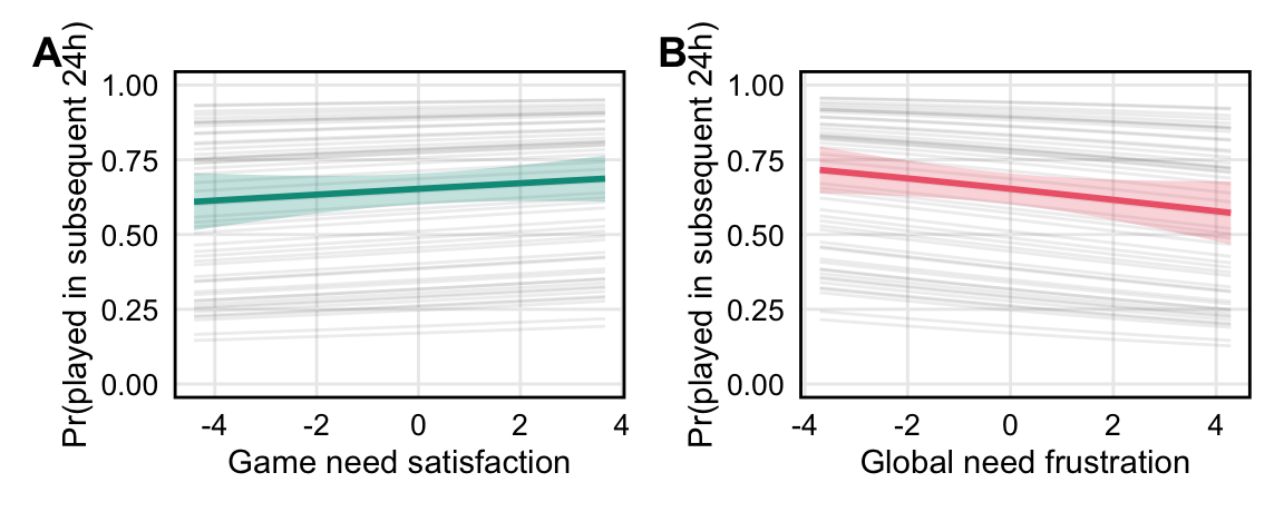
*H2a. When individuals’ in-game need satisfaction is higher, they are more likely to play video games in the 24-hour period after survey completion.*
### Compensation (H2b)
SDT predicts that (global) need frustration results in compensatory behavior---people attempt to replenish needs that are not being met by altering their behavior [e.g., @SheldonEtAl2011twoprocess]. The potent need satisfaction offered by games constitute one way for people to compensate, particularly those who are highly engaged with gaming and have high gaming literacy [@BallouEtAl2022People]. The so-called "need density hypothesis" predicts that problematic or disordered gaming is most likely to occur when a person experiences high need satisfaction in games and high need frustration in other life domains [@RigbyRyan2011glued]. In other words, problematic gaming is theorized to occur, at least for some, due to a negative feedback loop whereby compensation occurs and becomes maladaptive such that the person's other compensatory tools besides gaming are progressively diminished. Several studies have found support for the need density hypothesis account [@BradtEtAl2024Are; @AllenAnderson2018satisfaction; @MillsEtAl2018exploring].
BANG operationalizes this compensatory play via intrinsic motivation. Frustrated needs in one’s life in general make opportunities to fulfill those needs more salient, which---all else equal---manifests phenomenologically as a stronger preference towards activities that satisfy the frustrated need(s). Given this, we hypothesize in the context of our sample of moderately to highly-engaged video game players (derived from BANG Hypothesis 9):
*H2b. When individuals’ global need frustration is higher, they are more likely to play video games in the 24-hour period after survey completion.*
### Displacement (H3)
Playtime, BANG argues, only becomes problematic when it displaces other activities essential to the maintenance of need satisfaction in life overall. Commonly proposed problematic displacements are work/school responsibilities [@DrummondSauer2020Timesplitters], personal relationships [@DomahidiEtAl2018Longitudinal], and physical health or sleep [@KingEtAl2013impact]. Displacing these essential activities would thereby reduce global need satisfaction. Thus, BANG (B5) hypothesizes:
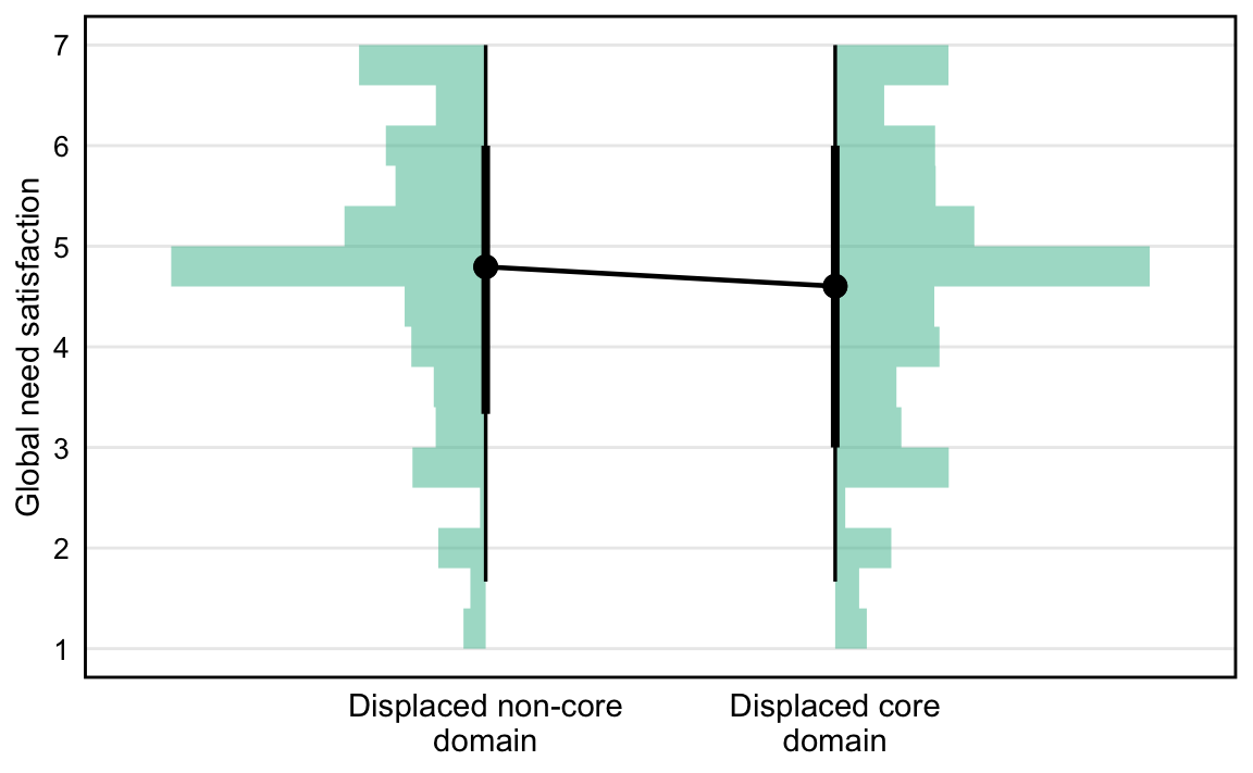
*H3. When a person’s most recent gaming is reported to displace a core life domain (work/school, social engagements, sleep/eating/fitness, or caretaking), their global need satisfaction is lower.*
# Study 1: Preregistered Analysis of Multi-Platform Digital Trace Data and Daily Surveys
Study 1 was pre-registered on the Open Science Framework (OSF) in the form of a Stage 1 Programmatic Registered Report [@BallouEtAl2025Psychological]. The present report is the first of three preregistered Stage 2 outputs; two other components, focused on sleep and genres, respectively, are forthcoming.
All data and analysis code are available on Zenodo ({{< meta data-url >}}).
## Study 1 Method
::: {.place arguments='top, scope: "parent", float: true'}
```{r}
#| label: tbl-platforms
#| code-summary: "Show code (Create platform details table)"
#| tbl-cap: "Platform Details"
tibble(
  Platform = c(
    "Nintendo",
    "Xbox",
    "Steam"
  ),
  `Data Source` = c(
    "Data-sharing agreements with Nintendo of America",
    "Data-sharing agreement with Microsoft",
    "Custom web app (Gameplay.Science)"
  ),
  `Account Linking Process` = c(
    "Participants shared an identifier contained within a QR code on the Nintendo web interface. Nintendo of America uses this identifier to retrieve gameplay data and share it with the research team.",
    "Participants consented to data sharing by opting in to the study on Xbox Insiders with their Xbox account. Microsoft retrieved and shared pseudonymized gameplay data for all consented accounts.",
    "Using a web app we developed (https://gameplay.science), participants consented to have their gameplay data monitored for the duration of the study. Authentication uses the official Steam API (OpenID)."
  ),
  `Type of Data Collected` = c(
    "Session records (what game was played, at what time, for how long) for first-party games only (games published in whole or in part by Nintendo).",
    "Session records (what game was played, at what time, for how long). Game titles were replaced with a random persistent identifier, but genre(s) and age ratings are shared.",
    "Hourly aggregates per game (every hour, the total time spent playing each game during the previous hour)"
  )
) |>
  tt(
    escape = TRUE,
    notes = list(
      "a" = list(
        i = 1,
        j = 3,
        text = "See https://accounts.nintendo.com/qrcode."
      ),
      "b" = list(
        i = 1,
        j = 4,
        text = "Nintendo-published games accounted for 63% of Switch playtime in our sample."
      ),
      "c" = list(
        i = 2,
        j = 3,
        text = "See https://support.xbox.com/en-US/help/account-profile/manage-account/guide-to-insider-program."
      )
    )
  ) |>
  style_tt(fontsize = 0.7) |>
  style_tt(i = 0, bold = TRUE, align = "c")
```
:::
### Design
The data for this study comprise a subset of the data from the Open Play study [@BallouEtAl2025Open], version 1.0.0. In the Open Play study, participants provided access to automated records of their gaming history on one or more platforms (Xbox, Steam, Nintendo Switch, iOS, Android) and completed an intake survey followed by a 30-day daily diary study. The intake survey included demographic questions and baseline measures of wellbeing. Daily data was collected between Oct 2024 and Aug 2025.
Participants were recruited in collaboration with two panel providers, Prolific and PureProfile. Participants were eligible if they were aged 18 or older, resided in the United States, self-reported playing video games for at least 1 hour per week, of which 50% must take place on eligible platforms (Nintendo, Xbox, and Steam), and successfully linked at least one gaming account on Xbox, Steam, and/or Nintendo Switch with validated recent digital trace data. iOS and Android data were collected but are not used in this analysis. For full details of the recruitment procedures and study methodology, see [@BallouEtAl2025Open].
### Ethics
This study received ethical approval from the Social Sciences and Humanities Inter-Divisional Research Ethics Committee at the University of Oxford (OII_CIA_23_107). All participants provided informed consent at the start of the study, including consent to their data being shared openly for reanalysis.
Participants were paid at an average rate of £12/hour, equating to: £0.20 for a 1-minute screening, £2 for the 10-minute intake survey (plus £5 for linking at least one account with recent data), £0.80 for each 4-minute daily survey. Participants received a £10 bonus payment for completing at least 24 out of 30 daily surveys.
### Sample Size Justification
As specified in the Stage 1 Registered Report, sample size was determined by feasibility/resources rather than a formal power analysis, with an initial target of recruiting up to 1,000 U.S. participants into the diary component, with ~30% expected attrition. Sensitivity analyses showed that this sample size was sufficient to estimate target associations with moderate precision (95% CI spanning .13 scale points on a 7-point scale) (https://github.com/digital-wellbeing/platform-study-rr).
### Participant Inclusion/Exclusion Criteria
All eligibility and exclusion criteria were specified prior to data analysis in Stage 1 and/or documented as deviations in @tbl-deviations. Participants were eligible if they were aged 18+, resided in the U.S., reported playing video games at least 1 hour/week, reported that a substantial share of their gaming occurred on eligible platforms (Nintendo/Xbox/Steam), and successfully linked at least one eligible account with validated recent digital trace data. As documented, two eligibility thresholds were adjusted for feasibility relative to Stage 1: the platform-share requirement was lowered (75% → 50%), and the recent valid trace requirement was extended (7 days → 14 days).
Participants who completed fewer than 15 daily surveys were excluded from the primary (imputed) analyses. The ≥15-survey threshold aligns with the Stage 1 criterion of avoiding analyses that would require imputing more data than collected (≥50%).
### Participants
```{r}
#| label: participants
#| code-summary: "Show code (Calculate participant statistics and response rates)"
# Analytic sample (≥15 completions, used in imputed analyses)
analytic_pids <- dat |>
  filter(.imp == 1) |>
  distinct(pid) |>
  pull(pid)

# Prepare participant data with collapsed categories
participant_data <- intake |>
  filter(pid %in% c(full_eligible_pids, analytic_pids)) |>
  mutate(
    # Collapse gender to main categories
    gender = ifelse(
      gender %in% c("Man", "Woman"),
      gender,
      "Other gender identity"
    ),
    # Collapse ethnicity to main categories
    ethnicity_collapsed = case_when(
      str_detect(ethnicity, "White") ~ "White",
      str_detect(
        ethnicity,
        "Black|African American|African, Caribbean"
      ) ~ "Black/African American",
      str_detect(ethnicity, "Asian") ~ "Asian",
      str_detect(ethnicity, "Two or More|Mixed") ~ "Multiracial",
      is.na(ethnicity) ~ NA_character_,
      TRUE ~ "Other"
    ),
    # Collapse education to main levels
    education_collapsed = case_when(
      str_detect(
        edu_level,
        "Less than|No formal|Primary"
      ) ~ "Less than high school",
      str_detect(
        edu_level,
        "High school|Secondary School|GCSE|Some college|Some University"
      ) ~ "High school or some college",
      str_detect(edu_level, "Associate") ~ "Associate degree",
      str_detect(
        edu_level,
        "Bachelor|University Bachelors"
      ) ~ "Bachelor's degree",
      str_detect(
        edu_level,
        "Master|Graduate|professional degree|doctoral|post-graduate"
      ) ~ "Graduate degree",
      is.na(edu_level) ~ NA_character_,
      TRUE ~ "Other"
    ),
    # Assign to sample
    sample = case_when(
      pid %in% analytic_pids ~ "Analytic sample",
      TRUE ~ "Full eligible sample"
    )
  ) |>
  select(
    pid,
    sample,
    age,
    gender,
    ethnicity_collapsed,
    education_collapsed,
    self_reported_weekly_play,
    diaries_completed
  )

# Sample sizes for text
n_analytic <- sum(participant_data$sample == "Analytic sample")
n_full <- sum(
  participant_data$sample %in% c("Analytic sample", "Full eligible sample")
)

# Gender summary for analytic sample (for text)
gender_analytic <- participant_data |>
  filter(sample == "Analytic sample") |>
  count(gender) |>
  mutate(pct = 100 * n / sum(n))

pct_men <- gender_analytic |> filter(gender == "Man") |> pull(pct) |> round(1)
pct_women <- gender_analytic |>
  filter(gender == "Woman") |>
  pull(pct) |>
  round(1)
pct_other <- gender_analytic |>
  filter(gender == "Other gender identity") |>
  pull(pct) |>
  round(1)

gender_summary <- glue(
  "{pct_men}% men, {pct_women}% women, {pct_other}% other gender identities"
)
```
```{r}
#| label: tbl-participants
#| tbl-cap: "Participant characteristics by sample"
#| code-summary: "Show code (Generate participant demographics table)"
# Build table using map
summary_table <- bind_rows(
  # Sample sizes
  tibble(
    Characteristic = "**N**",
    `Full sample` = as.character(n_full),
    `Analytic sample` = as.character(n_analytic)
  ),

  # Age
  tibble(
    Characteristic = "Age (years)",
    `Full sample` = format_mean_sd(
      participant_data$age[participant_data$sample == "Full eligible sample"]
    ),
    `Analytic sample` = format_mean_sd(
      participant_data$age[participant_data$sample == "Analytic sample"]
    )
  ),

  # Categorical demographics
  create_categorical_section(
    participant_data,
    "gender",
    "Gender",
    c("Man", "Woman", "Other gender identity")
  ),

  create_categorical_section(
    participant_data,
    "ethnicity_collapsed",
    "Ethnicity",
    c("White", "Black/African American", "Asian", "Multiracial", "Other")
  ),

  create_categorical_section(
    participant_data,
    "education_collapsed",
    "Education",
    c(
      "Less than high school",
      "High school or some college",
      "Associate degree",
      "Bachelor's degree",
      "Graduate degree"
    )
  ),

  # Gaming behavior section
  tibble(
    Characteristic = "**Gaming behavior**",
    `Full sample` = "",
    `Analytic sample` = ""
  ),

  tibble(
    Characteristic = "Weekly play (hours)",
    `Full sample` = format_mean_sd(
      participant_data$self_reported_weekly_play[
        participant_data$sample == "Full eligible sample"
      ] /
        60
    ),
    `Analytic sample` = format_mean_sd(
      participant_data$self_reported_weekly_play[
        participant_data$sample == "Analytic sample"
      ] /
        60
    )
  ),

  # Study engagement section
  tibble(
    Characteristic = "**Study engagement**",
    `Full sample` = "",
    `Analytic sample` = ""
  ),

  tibble(
    Characteristic = "Surveys completed",
    `Full sample` = format_mean_sd(
      participant_data$diaries_completed[
        participant_data$sample == "Full eligible sample"
      ]
    ),
    `Analytic sample` = format_mean_sd(
      participant_data$diaries_completed[
        participant_data$sample == "Analytic sample"
      ]
    )
  )
)

# Identify rows for styling
header_rows <- which(
  str_detect(summary_table$Characteristic, "^\\*\\*") |
    (summary_table$`Full sample` == "" & summary_table$`Analytic sample` == "")
)
indent_rows <- which(str_detect(summary_table$Characteristic, "^    "))

# Create table
summary_table |>
  tt(
    notes = "Values are M (SD) or N (%). Ethnicity and education categories collapsed to main levels for clarity."
  ) |>
  format_tt(j = 1, markdown = TRUE) |>
  style_tt(i = header_rows, bold = TRUE) |>
  format_tt(i = header_rows, j = 1, fn = function(x) {
    str_remove_all(x, "\\*\\*")
  }) |>
  style_tt(i = indent_rows, j = 1, indent = 1) |>
  format_tt(i = indent_rows, j = 1, fn = function(x) str_trim(x)) |>
  style_tt(fontsize = 0.7) |>
  style_tt(i = 0, bold = TRUE)
```
The current sample included `r n_analytic` participants (`r gender_summary`) who completed at least 15 daily surveys and were included in the main imputed analyses. The full eligible sample comprised `r n_full` participants who completed at least 1 survey and were included in complete case sensitivity analyses.
::: {.place arguments='top, scope: "parent", float: true'}
```{r}
#| label: fig-descriptives
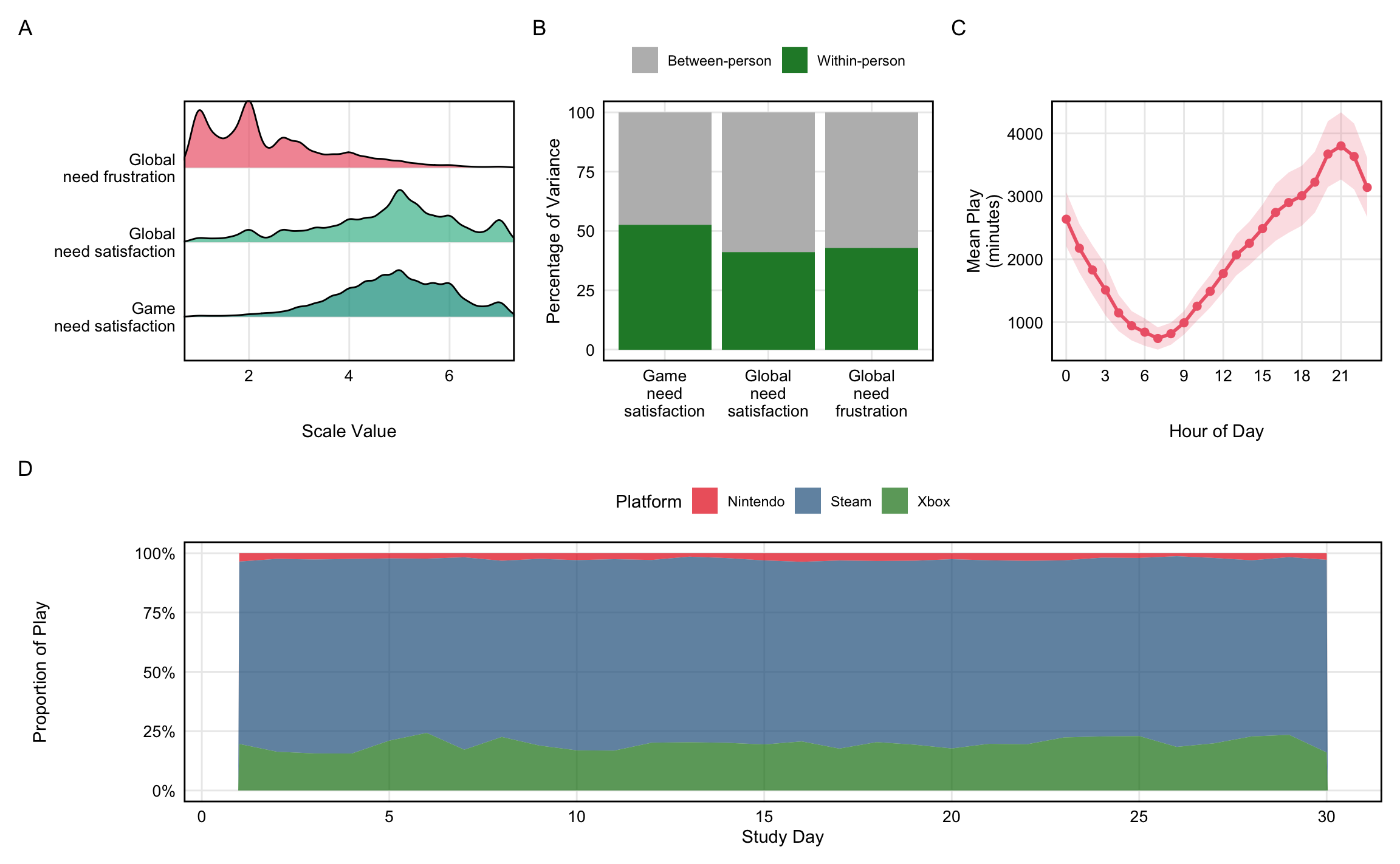
#| fig-cap: "Descriptive statistics for key variables. (A) Distributions of need satisfaction and frustration variables. (B) Variance decomposition showing proportion of variance at within-person vs between-person levels. (C) Play volume by hour of day (local time). (D) Proportion of play on each platform across study days 1-30."
#| code-summary: "Show code (Create main descriptive figure)"
#| fig-height: 8
#| fig-width: 12
# Panel A: Density ridges for key variables
dat_desc <- dat |> filter(.imp == 1)

panel_a <- dat_desc |>
  select(global_ns, global_nf, game_ns) |>
  pivot_longer(everything(), names_to = "variable", values_to = "value") |>
  mutate(
    variable = factor(
      variable,
      levels = c("game_ns", "global_ns", "global_nf"),
      labels = c(
        sub(" ", "\n", labels["game_ns"]),
        sub(" ", "\n", labels["global_ns"]),
        sub(" ", "\n", labels["global_nf"])
      )
    )
  ) |>
  ggplot(aes(x = value, y = variable, fill = variable)) +
  geom_density_ridges(alpha = 0.7, scale = 0.9, na.rm = TRUE) +
  scale_fill_manual(
    values = setNames(
      c(colors$game_ns, colors$global_ns, colors$global_nf),
      c(
        sub(" ", "\n", labels["game_ns"]),
        sub(" ", "\n", labels["global_ns"]),
        sub(" ", "\n", labels["global_nf"])
      )
    )
  ) +
  labs(x = "Scale Value", y = NULL) +
  coord_cartesian(xlim = c(1, 7)) +
  theme(legend.position = "none")

# Panel B: Variance decomposition
panel_b <- dat_desc |>
  select(pid, global_ns, global_nf, game_ns) |>
  pivot_longer(
    c(global_ns, global_nf, game_ns),
    names_to = "variable",
    values_to = "value"
  ) |>
  group_by(variable) |>
  summarise(
    var_total = var(value, na.rm = TRUE),
    var_between = var(tapply(value, pid, mean, na.rm = TRUE), na.rm = TRUE),
    .groups = "drop"
  ) |>
  mutate(
    pct_between = 100 * var_between / var_total,
    pct_within = 100 * (var_total - var_between) / var_total,
    variable = factor(
      variable,
      levels = c("game_ns", "global_ns", "global_nf"),
      labels = c(
        gsub(" ", "\n", labels["game_ns"]),
        gsub(" ", "\n", labels["global_ns"]),
        gsub(" ", "\n", labels["global_nf"])
      )
    )
  ) |>
  pivot_longer(
    c(pct_within, pct_between),
    names_to = "component",
    values_to = "percentage"
  ) |>
  mutate(
    component = factor(
      component,
      levels = c("pct_between", "pct_within"),
      labels = c(labels["Between-person"], labels["Within-person"])
    )
  ) |>
  ggplot(aes(x = variable, y = percentage, fill = component)) +
  geom_col(position = "stack") +
  scale_fill_manual(
    values = c(
      "Between-person" = colors$between,
      "Within-person" = colors$within
    )
  ) +
  labs(x = NULL, y = "Percentage of Variance", fill = NULL) +
  theme(legend.position = "top")

# Panel C: Hour of day patterns
panel_c <- hourly_telemetry |>
  filter(pid %in% unique(dat_desc$pid)) |>
  mutate(hour = hour(hour_start_local)) |>
  group_by(pid, hour) |>
  summarise(total_minutes = sum(minutes, na.rm = TRUE), .groups = "drop") |>
  group_by(hour) |>
  summarise(
    mean_minutes = mean(total_minutes, na.rm = TRUE),
    se = sd(total_minutes, na.rm = TRUE) / sqrt(n()),
    .groups = "drop"
  ) |>
  ggplot(aes(x = hour, y = mean_minutes)) +
  geom_ribbon(
    aes(ymin = mean_minutes - 1.96 * se, ymax = mean_minutes + 1.96 * se),
    fill = colors$global_nf,
    alpha = 0.2
  ) +
  geom_line(color = colors$global_nf, linewidth = 1) +
  geom_point(color = colors$global_nf, size = 2) +
  labs(x = "Hour of Day", y = "Mean Play\n(minutes)") +
  scale_x_continuous(breaks = seq(0, 23, 3))

# Panel D: Platform usage over study days
panel_d <- daily_telemetry |>
  mutate(day_local_date = as.Date(day_local)) |>
  inner_join(
    dat_desc |>
      select(pid, date, wave) |>
      mutate(
        date_only = as.Date(date),
        wave_num = as.numeric(as.character(wave))
      ) |>
      filter(wave_num <= 30),
    by = c("pid", "day_local_date" = "date_only"),
    relationship = "many-to-many"
  ) |>
  filter(minutes > 0) |>
  mutate(
    platform = case_when(
      platform == "nintendo" ~ "Nintendo",
      platform == "xbox" ~ "Xbox",
      platform == "steam" ~ "Steam",
      TRUE ~ platform
    )
  ) |>
  group_by(wave_num, platform) |>
  summarise(total_minutes = sum(minutes), .groups = "drop") |>
  group_by(wave_num) |>
  mutate(proportion = total_minutes / sum(total_minutes)) |>
  ggplot(aes(x = wave_num, y = proportion, fill = platform)) +
  geom_area(alpha = 0.7, position = "stack") +
  scale_fill_manual(
    values = c(
      "Nintendo" = colors$nintendo,
      "Xbox" = colors$xbox,
      "Steam" = colors$steam
    )
  ) +
  labs(x = "Study Day", y = "Proportion of Play", fill = "Platform") +
  scale_x_continuous(breaks = seq(0, 30, 5)) +
  scale_y_continuous(labels = scales::percent_format()) +
  theme(legend.position = "top")

# Combine panels: top row with 3 panels, bottom row with full-width panel
((panel_a | panel_b | panel_c) / panel_d) +
  plot_annotation(tag_levels = "A") &
  theme(
    plot.background = element_rect(fill = "white", color = NA),
    panel.background = element_rect(fill = "white", color = NA)
  )
```
:::
### Measures
```{r}
#| label: psychometrics
#| code-summary: "Show code (Calculate reliability for all scales)"
#| output: false
omega_global_ns <- number(
  omega(
    surveys |> select(bpnsfs_1, bpnsfs_3, bpnsfs_5),
    plot = FALSE
  )$omega.tot,
  .01
)
omega_global_nf <- number(
  omega(
    surveys |> select(bpnsfs_2, bpnsfs_4, bpnsfs_6),
    plot = FALSE
  )$omega.tot,
  .01
)

omega_game_ns <- number(
  omega(
    surveys |> select(bangs_1, bangs_3, bangs_5),
    plot = FALSE
  )$omega.tot,
  .01
)
omega_game_nf <- number(
  omega(
    surveys |> select(bangs_2, bangs_4, bangs_6),
    plot = FALSE
  )$omega.tot,
  .01
)

# proportion of surveys with subsequent play

prop_subsequent_play <- number(
  nrow(surveys[surveys$telemetry_played_any_24h, ]) / nrow(surveys) * 100,
  .1
)
minutes_subsequent_play <- number(
  mean(surveys$play_minutes_24h, na.rm = TRUE),
  1
)
sd_minutes_subsequent_play <- number(
  sd(surveys$play_minutes_24h, na.rm = TRUE),
  1
)

# total hours per platform during 30-day study period

platform_hours <- daily_telemetry |>
  mutate(day_local_date = as.Date(day_local)) |>
  inner_join(
    surveys |>
      select(pid, date, wave) |>
      distinct() |>
      mutate(
        date_only = as.Date(date),
        wave_num = as.numeric(as.character(wave))
      ) |>
      filter(wave_num <= 30),
    by = c("pid", "day_local_date" = "date_only"),
    relationship = "many-to-many"
  ) |>
  group_by(platform) |>
  summarise(total_hours = sum(minutes, na.rm = TRUE) / 60, .groups = "drop")

hours_nintendo <- number(
  platform_hours |> filter(platform == "Nintendo") |> pull(total_hours),
  1,
  big.mark = ","
)
hours_xbox <- number(
  platform_hours |> filter(platform == "Xbox") |> pull(total_hours),
  1,
  big.mark = ","
)
hours_steam <- number(
  platform_hours |> filter(platform == "Steam") |> pull(total_hours),
  1,
  big.mark = ","
)
```
The measures used in this paper are visualized in @fig-descriptives and detailed below. For other measures in the Open Play study not used here, we refer readers to the Open Play codebook [@BallouEtAl2025Open].
*Need satisfaction in games*. We measured need satisfaction and frustration in games during the most recent gaming session using 3 items from an abbreviated version of the Basic Psychological Need Satisfaction in Gaming Scale [BANGS, @BallouDeterding2024Basic]. The BANGS assesses autonomy, competence, and relatedness need satisfaction with three items for each need; we selected the highest-loading item for each need for our brief daily measure (e.g., relatedness satisfaction: "I felt I formed relationships with other players and/or characters."). Participants rated each item on a Likert scale from 1 (Strongly disagree) to 7 (Strongly agree). We calculated mean scores for need satisfaction by averaging all three items. Reliability of the composite 3-item need satisfaction index was assessed using McDonald’s omega total ($\omega_t$ = `r omega_game_ns` for need satisfaction, $\omega_t$ `r omega_game_nf` for need frustration). As needs are conceptually distinct, we expect lower reliability for the composite index than for unidimensional scales.
*Need satisfaction and frustration in daily life*. We measured need satisfaction and frustration in daily life ("global need satisfaction and frustration") during the previous 24 hours using the brief version of the Basic Psychological Need Satisfaction and Frustration Scale [@ChenEtAl2015Basic; @MartelaRyan2024Assessing]. This scale includes 6 items, with one item for need satisfaction and one item for need frustration for each of the three needs (e.g., "Today ... I was able to do things that I really want and value in life"). Participants rated each item on a Likert scale from 1 (Strongly disagree) to 7 (Strongly agree). We calculated mean scores for need satisfaction and need frustration by averaging the relevant items. Reliability of the composite 3-item need satisfaction index was assessed using McDonald’s omega total ($\omega_t$ = `r omega_global_ns` for need satisfaction; $\omega_t$ = `r omega_global_nf` for need frustration). As needs are conceptually distinct, we expect lower reliability for this composite index than for unidimensional scales.
*Video game playtime*. We measured video game playtime using digital trace data collected from participants' gaming accounts on Xbox, Steam, and Nintendo Switch. During the 30-day study period, we recorded a total of `r hours_nintendo` hours of play on Nintendo Switch, `r hours_xbox` hours on Xbox, and `r hours_steam` hours on Steam. For each daily survey, we calculated total minutes played in the 24-hour period following survey completion. We also created a binary variable indicating whether any play occurred during this period. On average, `r prop_subsequent_play`% of surveys were followed by any play in the subsequent 24 hours, with a mean of `r minutes_subsequent_play` minutes (SD = `r sd_minutes_subsequent_play`).
*Displacement*: We measured displacement of core life domains via an open text field asking participants about the hypothetical alternative activity: "Think back to your most recent gaming session. If you hadn't played a game, what would you most likely have done instead?" With LLM assistance from Qwen3-4b-instruct [@qwen3technicalreport], we coded participant responses based on whether they mentioned any of the following activities: work/school responsibilities, social engagements, sleep/eating/fitness, or caretaking---so-called "core life domains". We refined the LLM prompt through 5 iterations of manual verification of the 100 random coded responses. We created a boolean variable indicating whether any core life domain was hypothetically displaced. Full materials are provided in the supplement, including the exact LLM prompt used for classification, all raw participant responses, coded outputs, manual verification results, and reproducible code.
### Data Exclusions
Consistent with Stage 1, we applied preregistered exclusions to telemetry records prior to analysis: we excluded telemetry days with >16 hours total logged play across linked platforms, sessions >8 hours, and sessions logged in the future (indicating logging error or system-clock manipulation). We also excluded survey responses failing the preregistered attention check (duplicate need item responses differing by >1 scale point). As part of preregistered data quality processing, we removed background sessions and verified there were no overlapping sessions after preprocessing, before proceeding to the planned analyses. No additional exclusion criteria beyond those preregistered were introduced.
### Imputation
We used multiple imputation by chained equations (MICE) with predictive mean matching (PMM) to handle missing data. Missing data were imputed for daily need satisfaction/frustration items (BPNSFS, BANGS) and displacement measures (an average of `r overall_miss_pct`% missing cells across `r pct_ppl_with_missing`% of participants with at least one wave of missing data). Digital trace data were not imputed because tracking was continuous and automatic; within-platform, missing data represent recorded absence of play.
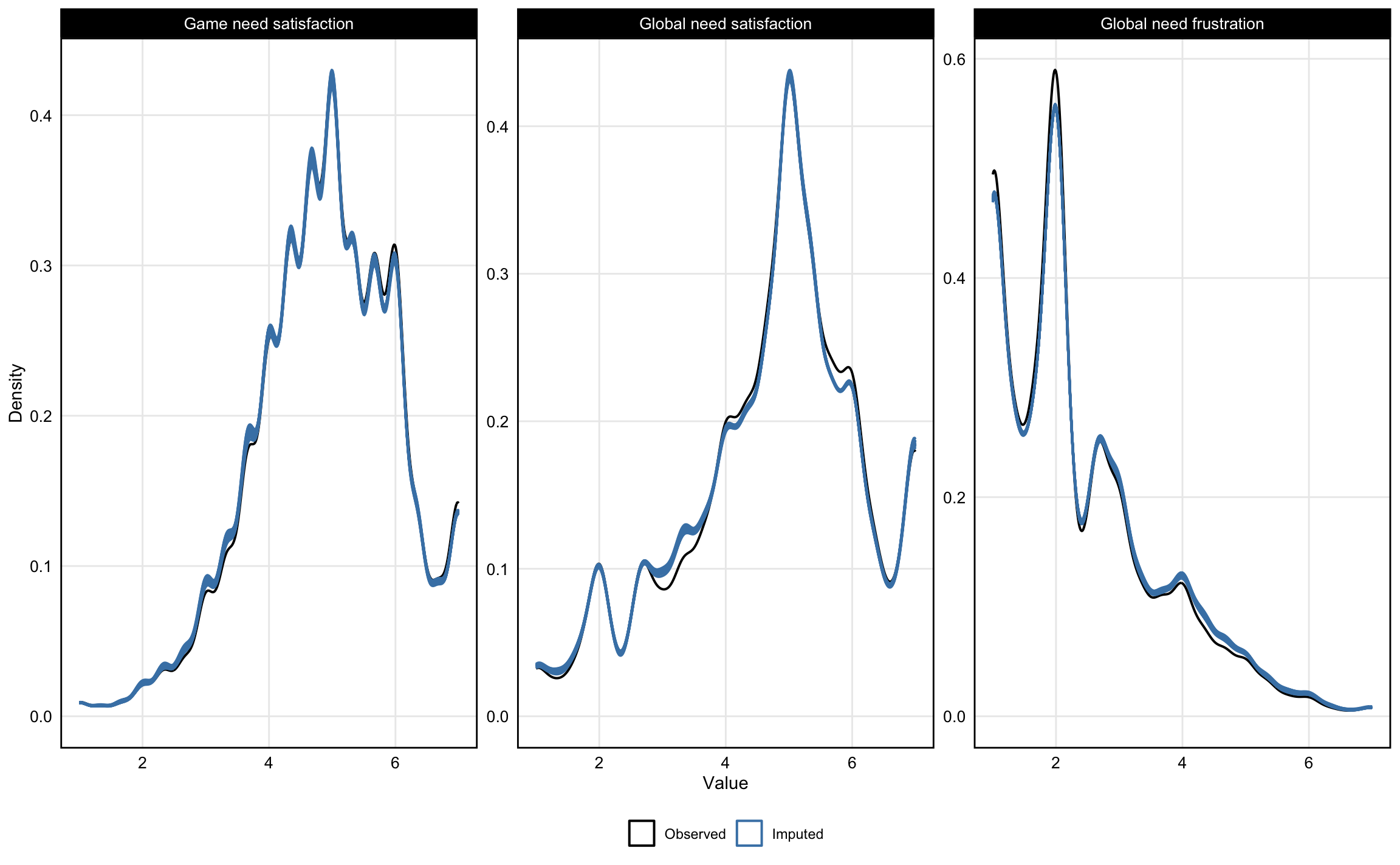
Following the two-stage protocol from @VonHippel2020How based on fraction of missing information, we used 27 imputations. For all variables, imputed distributions closely overlapped with the observed data (see Appendix @fig-imputation). Models were fit separately to each imputed dataset, and estimates were pooled across imputations using Rubin's rules as implemented in the `mice` package [@vanBuurenGroothuis-Oudshoorn2011mice]. For comparison, complete case analyses are reported in the Appendix (Sensitivity Analysis 4); results do not meaningfully differ from the imputed analyses.
### Deviations from Preregistration
We made several deviations from our preregistration to ensure we could recruit enough high-quality participants to meet our sample size goals. In our view, none are so severe enough to threaten the validity of the study. Deviations are summarized in @tbl-deviations.
::: {.place arguments='top, scope: "parent", float: true'}
```{r}
#| label: tbl-deviations
#| code-summary: "Show code (Create table of preregistration deviations)"
#| tbl-cap: "Summary of deviations from preregistration"
tibble(
  `Study Aspect` = c(
    "Data collection",
    "Data collection",
    "Data collection",
    "Data collection",
    "Data collection",
    "Data collection",
    "Analysis"
  ),
  Preregistered = c(
    "All participants sourced from PureProfile",
    "Screening sample would be nationally representative by ethnicity and gender",
    "Sample consists of participants aged 18--30",
    "To qualify, >=75% of a participant's total gaming must take place on platforms included in the study (Xbox, Steam, Nintendo Switch)",
    "Qualification contingent upon valid digital trace data within last 7 days",
    "Daily surveys sent at 7pm local time",
    "Data would be imputed for all participants given a 50% overall response rate"
  ),
  Actual = c(
    "Participants sourced from both PureProfile and Prolific",
    "Approximately 50% of screening was done using quotas for national representativeness by ethnicity and gender; all subsequent sampling used convenience sampling with no quotas",
    "Sample consists of participants aged 18-40",
    "To qualify, >=50% of a participant's total gaming must take place on platforms included in the study (Xbox, Steam, Nintendo Switch)",
    "Qualification contingent upon valid digital trace data within last 14 days",
    "Daily surveys sent at 2pm local time",
    "Data imputed for only participants with an individual 50% response rate"
  ),
  `Justification for Deviation` = c(
    "Exhausted PureProfile participant pool before reaching required sample size",
    "Exhausted participant pools of smaller demographic categories on both Prolific and PureProfile before reaching required sample size",
    "(1) Unable to recruit enough participants in the US aged 18--30",
    "Low rates of study qualification at 75% threshold, in large part due to substantial uncaptured Playstation play",
    "Feedback from participants indicating that play during a 7-day period was subject to too many fluctuations (e.g., a busy workweek)",
    "Feedback from participants indicating that evening plans often interfered with survey completion and thus adversely affected response rate",
    "Imputing values for participants with 50--97% missing data is poorly justified; results from the preregistered analysis with imputation for all participants are reported in the Appendix (Sensitivity Analysis 5) and do not meaningfully differ from the main analysis"
  )
) |>
  tt() |>
  style_tt(fontsize = 0.7) |>
  style_tt(i = 0, bold = TRUE, align = "c")
```
:::
### Positive Controls
```{r}
#| label: positive-controls
#| code-summary: "Show code (Test positive controls)"
# Use first imputation for positive control check
cor_playtime <- cor.test(
  dat$self_reported_weekly_play[dat$.imp == 1],
  dat$play_minutes_24h[dat$.imp == 1],
  method = "pearson"
)

cor_playtime_inline <- glue(
  "r = {number(cor_playtime$estimate, .01)}, 95% CI [{number(cor_playtime$conf.int[1], .01)}, {number(cor_playtime$conf.int[2], .01)}]"
)
```
As specified in the preregistration, we assessed two positive controls designed to assess whether our data were capable of addressing our stated hypotheses. Both passed: self-reported playtime correlated positively with logged playtime (`r cor_playtime_inline`); and after preprocessing (e.g., to remove background sessions), there were no overlapping sessions. We therefore proceeded with the planned analyses.
### Analysis Approach
We tested each hypothesis using multilevel within-between regression models estimated with `glmmTMB` [@BrooksEtAl2017glmmTMB]. Focal predictors were within-person mean-centered, with 30-day person means included to separate day-level from 30-day aggregate associations. All models included random intercepts and AR(1) autocorrelation structures; H1 and H3 additionally included random slopes for day-level predictors, while H2 used random intercepts only due to convergence issues with the binary outcome. No demographic covariates were included, as the within-between specification controls for all time-invariant individual differences.
This approach isolates day-to-day dynamics: day-level coefficients estimate how much a person's outcome deviates from their own 30-day average when their predictor deviates from their own 30-day average. For example, H1's day-level coefficient answers: 'On days when individuals experience better game need satisfaction than their typical level, do they report higher global need satisfaction than their typical level?' The non-focal 30-day aggregate coefficients capture whether people with generally higher predictor levels also have generally higher outcomes across the study period. Random effects account for stable individual differences (e.g., personality, gaming preferences), and the AR(1) term models temporal autocorrelation in daily data. This specification does not adjust for time-varying confounds; estimates should be interpreted as associations rather than causal effects.
## Study 1 Results: Confirmatory
We present visualizations for each hypothesis test in turn; all key estimates are summarized @tbl-main-results.
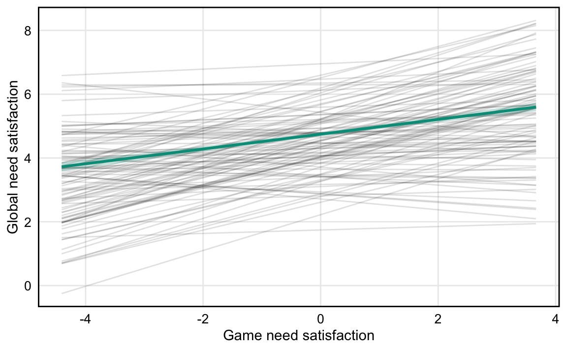
### H1. Greater in-game need satisfaction is associated with greater global need satisfaction
```{r}
#| label: h1-model
#| output: false
#| code-summary: "Show code (Fit H1 models: game NS → global NS)"
# File-based caching to avoid re-running across multiple output formats
h1_cache_file <- "data/models/h1_fits.rds"
h1_pooled_file <- "data/models/h1_pooled.rds"

if (file.exists(h1_cache_file) && file.exists(h1_pooled_file)) {
  message("Loading cached H1 model fits")
  h1_fits <- readRDS(h1_cache_file)
  h1_pooled <- readRDS(h1_pooled_file)
  h1mod <- h1_fits[[1]]
} else {
  message("Fitting H1 models...")

  # Fit model to each imputed dataset
  h1_fits <- lapply(1:m_imputations, function(i) {
    message(glue("Fitting H1 model to imputation {i} of {m_imputations}"))
    dat_i <- dat |> filter(.imp == i)
    glmmTMB(
      global_ns ~ game_ns_cw +
        game_ns_cb +
        (1 + game_ns_cw | pid) +
        ar1(wave + 0 | pid),
      data = dat_i
    )
  })

  # Pool estimates using Rubin's rules
  h1_pooled <- pool(h1_fits)

  # Use first imputation's model for plotting
  h1mod <- h1_fits[[1]]

  # Save results
  dir.create("data/models", showWarnings = FALSE, recursive = TRUE)
  saveRDS(h1_fits, h1_cache_file)
  saveRDS(h1_pooled, h1_pooled_file)
  message("Saved H1 model fits to cache")
}
```
```{r}
#| label: h1-diagnostics
#| code-summary: "Show code (Check H1 model diagnostics and convergence)"
#| eval: !expr interactive()
# Convergence check across imputations
conv_summary <- tibble(
  imputation = seq_along(h1_fits),
  converged = map_lgl(h1_fits, ~ .x$fit$convergence == 0),
  warnings = map_chr(
    h1_fits,
    ~ {
      w <- .x$fit$warnings
      if (length(w) > 0) paste(w, collapse = "; ") else "None"
    }
  )
)
print(conv_summary)
glue("Converged: {sum(conv_summary$converged)}/{nrow(conv_summary)}")

# Random effect structure (from converged models)
re_sd <- attr(VarCorr(h1mod)$cond$pid, "stddev")
glue("Random intercept SD: {round(re_sd[1], 3)}")
if (length(re_sd) > 1) {
  glue("Random slope SD (game_ns_cw): {round(re_sd[2], 3)}")
}
```
```{r}
#| label: tbl-h1-results
#| include: false
#| code-summary: "Show code (Extract H1 estimates for inline text)"
# Extract estimates for narrative reporting
h1_summary <- summary(h1_pooled) |> as_tibble()
h1_ests <- report_wb_estimate(
h1_summary,
"game_ns_cw",
"game_ns_cb",
accuracy = 0.01
)
# Individual variables for inline reporting
h1_day_est <- h1_ests$day_level
h1_day_coef <- h1_ests$day_coef
h1_agg_est <- h1_ests$aggregate
h1_agg_coef <- h1_ests$agg_coef
h1_results <- h1_summary |>
select(term, estimate, std.error, statistic, p.value) |>
mutate(
term = ifelse(term %in% names(labels), labels[term], term),
across(c(estimate, std.error, statistic), ~ round(.x, 3))
)
```
::: {.place arguments='top, scope: "parent", float: true'}
```{r}
#| label: fig-h1-predictions
#| fig-cap: "Estimated global need satisfaction as a function of need satisfaction in games. Individual trajectories shown as gray lines, population-level association shown as blue line with 95% confidence ribbon."
#| code-summary: "Show code (Plot H1)"
plot_relationship(
  model = h1mod,
  x_var = "game_ns_cw",
  x_label = labels["game_ns"],
  y_label = labels["global_ns"],
  color = colors$game_ns,
  n_keepers = 100,
  within_vars = c("game_ns_cw"),
  between_vars = c("game_ns_cb")
)
```
:::
Results strongly support H1 (@fig-h1-predictions). At the day level, game need satisfaction was positively associated with global need satisfaction (β = `r h1_day_est`). On days when participants experienced game need satisfaction 1 scale point (1--7 scale) above their personal 30-day average, they reported global need satisfaction `r h1_day_coef` units above their personal 30-day average.
At the 30-day aggregate level, which was not the focus of our hypothesis about day-to-day dynamics, the association (β = `r h1_agg_est`) was strong, indicating strong between-individual differences.
### H2. Situational need satisfaction is positively associated with the likelihood of playing in the period after survey completion (H2a), while global need frustration is negatively associated (H2b)
```{r}
#| label: h2-model
#| output: false
#| code-summary: "Show code (Fit H2 models: game NS + global NF → play)"
# File-based caching to avoid re-running across multiple output formats
h2_cache_file <- "data/models/h2_fits.rds"
h2_pooled_file <- "data/models/h2_pooled.rds"

if (file.exists(h2_cache_file) && file.exists(h2_pooled_file)) {
  message("Loading cached H2 model fits")
  h2_fits <- readRDS(h2_cache_file)
  h2_pooled <- readRDS(h2_pooled_file)
  h2mod <- h2_fits[[1]]
} else {
  message("Fitting H2 models...")

  # Fit model to each imputed dataset
  # Simplified: random intercept only + AR(1) for convergence
  h2_fits <- lapply(1:m_imputations, function(i) {
    message(glue("Fitting H2 model to imputation {i} of {m_imputations}"))
    dat_i <- dat |> filter(.imp == i)
    glmmTMB(
      telemetry_played_any_24h ~
        game_ns_cw +
        game_ns_cb +
        global_nf_cw +
        global_nf_cb +
        (1 | pid) +
        ar1(wave + 0 | pid),
      data = dat_i,
      family = binomial(link = "logit"),
      ziformula = ~0
    )
  })

  # Pool estimates using Rubin's rules
  h2_pooled <- pool(h2_fits)

  # Use first imputation's model for plotting
  h2mod <- h2_fits[[1]]

  # Save results
  dir.create("data/models", showWarnings = FALSE, recursive = TRUE)
  saveRDS(h2_fits, h2_cache_file)
  saveRDS(h2_pooled, h2_pooled_file)
  message("Saved H2 model fits to cache")
}

# Extract estimates for narrative reporting
h2_summary <- summary(h2_pooled) |> as_tibble()

# H2a: Game need satisfaction
h2a_ests <- report_wb_estimate(
  h2_summary,
  "game_ns_cw",
  "game_ns_cb",
  accuracy = 0.01
)
h2a_day_est <- h2a_ests$day_level
h2a_day_coef <- h2a_ests$day_coef
h2a_agg_est <- h2a_ests$aggregate
h2a_agg_coef <- h2a_ests$agg_coef

# H2b: Global need frustration
h2b_ests <- report_wb_estimate(
  h2_summary,
  "global_nf_cw",
  "global_nf_cb",
  accuracy = 0.01
)
h2b_day_est <- h2b_ests$day_level
h2b_day_coef <- h2b_ests$day_coef
h2b_agg_est <- h2b_ests$aggregate
h2b_agg_coef <- h2b_ests$agg_coef
```
```{r}
#| label: h2-diagnostics
#| code-summary: "Show code (Check H2 model diagnostics and convergence)"
#| eval: !expr interactive()
#| fig-width: 8
# Convergence check across imputations
conv_summary <- tibble(
  imputation = seq_along(h2_fits),
  converged = map_lgl(h2_fits, ~ .x$fit$convergence == 0),
  warnings = map_chr(
    h2_fits,
    ~ {
      w <- .x$fit$warnings
      if (length(w) > 0) paste(w, collapse = "; ") else "None"
    }
  )
)
print(conv_summary)
glue("Converged: {sum(conv_summary$converged)}/{nrow(conv_summary)}")

# Random effect structure (from converged models)
re_sd <- attr(VarCorr(h2mod)$cond$pid, "stddev")
re_names <- names(re_sd)
walk2(re_names, re_sd, ~ glue("{.x} SD: {round(.y, 3)}"))

# Random intercept distribution (logit scale)
re_intercepts <- coef(h2mod)$cond$pid[, "(Intercept)"]
tibble(
  stat = c("Mean", "SD", "Min", "Max", "IQR_25%", "IQR_75%"),
  value = c(
    mean(re_intercepts),
    sd(re_intercepts),
    min(re_intercepts),
    max(re_intercepts),
    quantile(re_intercepts, 0.25),
    quantile(re_intercepts, 0.75)
  )
) |>
  mutate(value = round(value, 3)) |>
  print()

# Implied probability at fixed intercept
fixed_int <- fixef(h2mod)$cond["(Intercept)"]
glue("Pr(play) at population mean: {round(plogis(fixed_int), 3)}")

# DHARMa residual diagnostics
sim_resid <- simulateResiduals(h2mod, plot = FALSE)

# Overall fit
plot(sim_resid, main = "H2 Model: DHARMa diagnostics")

# Statistical tests
list(
  dispersion = testDispersion(sim_resid),
  outliers = testOutliers(sim_resid),
  quantiles = testQuantiles(sim_resid)
) |>
  walk(print)

# Residuals vs. predictors
par(mfrow = c(2, 2))
walk2(
  c("game_ns_cw", "global_nf_cw", "game_ns_cb", "global_nf_cb"),
  c(
    labels["game_ns_cw"],
    labels["global_nf_cw"],
    labels["game_ns_cb"],
    labels["global_nf_cb"]
  ),
  ~ plotResiduals(sim_resid, form = h2mod$frame[[.x]], main = glue("vs. {.y}"))
)
par(mfrow = c(1, 1))

# Temporal autocorrelation (within-person lag-1)
acf_by_person <- h2mod$frame |>
  group_by(pid) |>
  arrange(wave) |>
  filter(n() >= 3) |>
  reframe(
    acf = cor(
      sim_resid$scaledResiduals[cur_group_rows()][-n()],
      sim_resid$scaledResiduals[cur_group_rows()][-1],
      use = "complete.obs"
    )
  ) |>
  pull(acf)

tibble(
  stat = c("Mean", "Median", "Min", "Max"),
  lag1_acf = c(
    mean(acf_by_person),
    median(acf_by_person),
    min(acf_by_person),
    max(acf_by_person)
  )
) |>
  mutate(lag1_acf = round(lag1_acf, 3)) |>
  print()

# Aggregated residuals
recalculateResiduals(sim_resid, group = h2mod$frame$wave) |>
  plot(main = "Residuals by wave")
recalculateResiduals(sim_resid, group = h2mod$frame$pid) |>
  plot(main = "Residuals by individual")
```
::: {.place arguments='top, scope: "parent", float: true'}
```{r}
#| label: fig-h2-predictions
#| fig-cap: "Estimated probability of playing in subsequent 24 hours. (A) As a function of need satisfaction in games (H2a). (B) As a function of global need frustration (H2b). Individual trajectories shown as gray lines, population-level associations shown with 95% confidence ribbons."
#| code-summary: "Show code (Plot H2)"
#| fig-asp: 0.4
# Panel A: Game need satisfaction
p_h2a <- plot_relationship(
  model = h2mod,
  x_var = "game_ns_cw",
  x_label = labels["game_ns"],
  y_label = "Pr(played in subsequent 24h)",
  color = colors$game_ns,
  n_keepers = 50,
  within_vars = c("game_ns_cw", "global_nf_cw"),
  between_vars = c("game_ns_cb", "global_nf_cb")
)

# Panel B: Global need frustration
p_h2b <- plot_relationship(
  model = h2mod,
  x_var = "global_nf_cw",
  x_label = labels["global_nf"],
  y_label = "Pr(played in subsequent 24h)",
  color = colors$global_nf,
  n_keepers = 50,
  within_vars = c("game_ns_cw", "global_nf_cw"),
  between_vars = c("game_ns_cb", "global_nf_cb")
)

# Combine with patchwork and set y-axis limits to 0-100%
p_h2a +
  p_h2b +
  plot_annotation(tag_levels = "A") &
  coord_cartesian(ylim = c(0, 1)) &
  theme(plot.tag = element_text(face = "bold", size = 14))
```
:::
We tested H2a and H2b using a single multilevel within-between logistic regression, where in-game need satisfaction and global need frustration (each within- and between-person centered) predicted a binary variable whether any play happened in the 24-hour period after diary survey completion.
Results support neither H2a or H2b: at the day level, experiencing neither 1 point higher game need satisfaction (β = `r h2a_day_est`) nor 1 point higher global need frustration (β = `r h2b_day_est`) than usual on a 1-point scale showed meaningful associations with the likelihood of subsequent play (see @fig-h2-predictions).
We conducted a wide range of sensitivity analyses providing convergent conclusions: key estimates for gaming need satisfaction (game NS) and global need frustration (global NF) remain indistinguishable from 0 in models that:
- use subsequent 6 hours (game NS: β = 0.04; global NF: β = -0.01) or 12 hours (game NS: β = 0.04; global NF: β = -0.02) as the outcome, instead of 24 hours (Sensitivity Analysis 1)
- use alternative random slopes specifications (game NS: β = 0.04; global NF: β = -0.06) (Sensitivity Analysis 2)
- use a count model of minutes played in the subsequent 24 hours instead of binary play/no-play (game NS: β = 0.04; global NF: β = -0.08) (Sensitivity Analysis 3)
- use complete case data instead of imputed data (game NS: β = 0.04; global NF: β = -0.08) (Sensitivity Analysis 4)
- impute data from the full eligible sample instead of the analytic sample (game NS: β = 0.04; global NF: β = -0.08) (Sensitivity Analysis 5)
- include an interaction between gaming need satisfaction and global need frustration (game NS: β = 0.04; global NF: β = -0.08; game NS * global NF: β = 0.04) (Sensitivity Analysis 6)
- use a spline term for gaming need satisfaction and global need frustration, instead of a linear term (Sensitivity Analysis 7)
- enter each individual need (autonomy, competence, relatedness) as predictors instead of composite need satisfaction or frustration (Sensitivity Analysis 8)
The 30-day aggregate associations (game need satisfaction: β = `r h2a_agg_est`; global need frustration: β = `r h2b_agg_est`) similarly indicate no relationship across individuals; these are reported as exploratory and unrelated to the focal hypotheses about short-term behavioral dynamics.
In short, results consistently fail to detect an association between situational need satisfaction or global need frustration and subsequent play behavior.
### H3. When gaming displaces a core life domain, global need satisfaction will be lower
```{r}
#| label: h3-displaced-categories
#| include: false
#| code-summary: "Show code (Calculate displaced activity category frequencies)"
# Calculate frequencies of each displaced activity category
# Use first imputation to avoid double-counting
activity_summary <- dat |>
filter(.imp == 1, !is.na(displaced_core_domain)) |>
left_join(
activity_categories |> select(pid, wave, activity_label),
by = c("pid", "wave")
) |>
count(activity_label, displaced_core_domain) |>
group_by(activity_label) |>
mutate(
pct = 100 * n / sum(n),
total = sum(n)
) |>
ungroup() |>
arrange(desc(total))
# Get counts for core vs non-core
core_summary <- dat |>
filter(.imp == 1, !is.na(displaced_core_domain)) |>
count(displaced_core_domain) |>
mutate(pct = 100 * n / sum(n))
# Store values for inline reporting (formatted)
total_responses <- scales::comma(sum(activity_summary$n))
n_core_raw <- core_summary |> filter(displaced_core_domain == TRUE) |> pull(n)
n_core <- scales::comma(n_core_raw)
pct_core <- round(
core_summary |> filter(displaced_core_domain == TRUE) |> pull(pct),
1
)
# Core domain specific counts
n_sleep <- scales::comma(
activity_summary |>
filter(activity_label == "sleep_eat_fitness") |>
pull(total) |>
first()
)
n_social <- scales::comma(
activity_summary |>
filter(activity_label == "social_engagement") |>
pull(total) |>
first()
)
n_work <- scales::comma(
activity_summary |>
filter(activity_label == "work_school") |>
pull(total) |>
first()
)
n_caretaking <- scales::comma(
activity_summary |>
filter(activity_label == "caretaking") |>
pull(total) |>
first()
)
# Non-core category counts for informal mention
n_digital_media <- scales::comma(
activity_summary |>
filter(activity_label == "other_digital_media") |>
pull(total) |>
first()
)
n_other_leisure <- scales::comma(
activity_summary |>
filter(activity_label == "other_leisure") |>
pull(total) |>
first()
)
```
```{r}
#| label: h3-model
#| output: false
#| code-summary: "Show code (Fit H3 models: displaced core domain → global NS)"
# File-based caching to avoid re-running across multiple output formats
h3_cache_file <- "data/models/h3_fits.rds"
h3_pooled_file <- "data/models/h3_pooled.rds"

if (file.exists(h3_cache_file) && file.exists(h3_pooled_file)) {
  message("Loading cached H3 model fits")
  h3_fits <- readRDS(h3_cache_file)
  h3_pooled <- readRDS(h3_pooled_file)
  h3mod <- h3_fits[[1]]
} else {
  message("Fitting H3 models...")

  # Fit model to each imputed dataset
  h3_fits <- lapply(1:m_imputations, function(i) {
    dat_i <- dat |> filter(.imp == i)
    glmmTMB(
      global_ns ~ displaced_core_domain +
        (1 + displaced_core_domain | pid) +
        ar1(wave + 0 | pid),
      data = dat_i
    )
  })

  # Pool estimates using Rubin's rules
  h3_pooled <- pool(h3_fits)

  # Use first imputation's model for plotting
  h3mod <- h3_fits[[1]]

  # Save results
  dir.create("data/models", showWarnings = FALSE, recursive = TRUE)
  saveRDS(h3_fits, h3_cache_file)
  saveRDS(h3_pooled, h3_pooled_file)
  message("Saved H3 model fits to cache")
}

# Extract estimates for narrative reporting
h3_summary <- summary(h3_pooled) |> as_tibble()
h3_ests <- report_wb_estimate(
  h3_summary,
  "displaced_core_domainTRUE",
  term_cb = NULL,
  accuracy = 0.01
)

h3_est <- h3_ests$day_level
h3_coef <- h3_ests$day_coef
```
::: {.place arguments='top, scope: "parent", float: true'}
```{r}
#| label: fig-h3-predictions
#| fig-cap: "Global need satisfaction when gaming was reported to displace vs. not displace a core life domain. Plot shows distribution (histogram) and mean with 80% and 95% quantile intervals."
#| code-summary: "Show code (Plot H3: displaced activity categories vs global NS)"
#| out-width: 60%
# Get raw data from first imputation for visualization
h3_data <- dat |>
  filter(.imp == 1, !is.na(displaced_core_domain)) |>
  mutate(
    displacement_label = if_else(
      displaced_core_domain,
      "Displaced core domain",
      "Displaced non-core domain"
    ),
    x_numeric = if_else(displaced_core_domain, 2, 1)
  )

# Calculate means for each group (to match what stat_histinterval will show)
h3_means <- h3_data |>
  group_by(x_numeric, displacement_label) |>
  summarise(mean_ns = mean(global_ns, na.rm = TRUE), .groups = "drop")

ggplot(h3_data, aes(x = x_numeric, y = global_ns)) +
  # Raincloud plot with asymmetric histograms
  stat_histinterval(
    data = h3_data |> filter(!displaced_core_domain),
    aes(fill = displacement_label),
    slab_alpha = 0.5,
    point_interval = mean_qi,
    breaks = seq(1, 7, by = .4),
    interval_color = "black",
    point_color = "black",
    point_size = 3,
    slab_fill = colors$global_ns,
    side = "left"
  ) +
  stat_histinterval(
    data = h3_data |> filter(displaced_core_domain),
    aes(fill = displacement_label),
    slab_alpha = 0.5,
    point_interval = mean_qi,
    breaks = seq(1, 7, by = .4),
    interval_color = "black",
    point_color = "black",
    point_size = 3,
    slab_fill = colors$global_ns,
    side = "right"
  ) +
  # Line connecting the mean point estimates
  geom_line(
    data = h3_means,
    aes(x = x_numeric, y = mean_ns),
    color = "black",
    linewidth = 0.8,
    linetype = "solid"
  ) +
  scale_x_continuous(
    breaks = c(1, 2),
    labels = c("Displaced non-core\ndomain", "Displaced core\ndomain")
  ) +
  scale_y_continuous(
    breaks = 1:7,
    limits = c(1, 7)
  ) +
  labs(
    x = NULL,
    y = labels["global_ns"]
  ) +
  theme(
    axis.text.x = element_text(size = 11),
    panel.grid.major.x = element_blank(),
    legend.position = "none"
  )
```
:::
Participants reported what activity their gaming session displaced `r total_responses` times across the study. In `r n_core` cases (`r pct_core`%), gaming displaced a core life domain: sleep, eating, or fitness (*n* = `r n_sleep`), social engagements (*n* = `r n_social`), work or school (*n* = `r n_work`), or caretaking (*n* = `r n_caretaking`). Gaming most commonly displaced non-core activities such as other digital media use (*n* = `r n_digital_media`) and other leisure activities (*n* = `r n_other_leisure`).
Results provide very weak support for H3 (β = `r h3_est`). When gaming displaced a core life domain rather than a non-core activity, participants reported global need satisfaction `r h3_coef` units lower on average. On a 7-point scale, this difference is extremely small, and the distributions of global need satisfaction when gaming displaced core vs. non-core domains are nearly identical (@fig-h3-predictions).
An exploratory analysis (Appendix Sensitivity Analysis 10) examined whether this relationship differed for specific displaced life domains. Results showed that need satisfaction was lower when gaming displaced work/school responsibilities and sleep/eating/fitness, but---contrary to expectations---tended to be higher when gaming displaced social engagements or caretaking. We return to this in the discussion.
```{r}
#| label: tbl-main-results
#| tbl-cap: "Summary of main hypothesis tests (H1-H3)"
#| code-summary: "Show code (Create combined results table)"
# Combine all three hypothesis results into one table
h1_combined <- summary(h1_pooled) |>
  as_tibble() |>
  filter(term != "(Intercept)", !str_detect(term, "_cb")) |>
  select(term, estimate, std.error, statistic, p.value) |>
  mutate(
    Model = "H1: game NS → global NS",
    term = ifelse(term %in% names(labels), labels[as.character(term)], term),
    test_stat = "t"
  )

h2_combined <- summary(h2_pooled) |>
  as_tibble() |>
  filter(term != "(Intercept)", !str_detect(term, "_cb")) |>
  select(term, estimate, std.error, statistic, p.value) |>
  mutate(
    Model = "H2: game NS + global NF → play",
    term = ifelse(term %in% names(labels), labels[term], term),
    test_stat = "z"
  )

h3_combined <- summary(h3_pooled) |>
  as_tibble() |>
  filter(term != "(Intercept)") |>
  select(term, estimate, std.error, statistic, p.value) |>
  mutate(
    Model = "H3: displaced core → global NS",
    term = ifelse(term %in% names(labels), labels[term], term),
    test_stat = "t"
  )

# Combine and format
bind_rows(h1_combined, h2_combined, h3_combined) |>
  mutate(
    across(c(estimate, std.error, statistic), ~ round(.x, 3)),
    p.value = case_when(
      p.value < 0.001 ~ "<.001",
      TRUE ~ as.character(round(p.value, 3))
    ),
    # Create combined test statistic column with appropriate label
    test_result = glue("{statistic} ({test_stat})")
  ) |>
  select(
    Model,
    Parameter = term,
    Estimate = estimate,
    SE = std.error,
    `Statistic` = test_result,
    `p` = p.value
  ) |>
  tt() |>
  style_tt(fontsize = 0.7) |>
  style_tt(i = 0, bold = TRUE) |>
  group_tt(j = "Model")
```
# Study 2: Exploratory Evidence from PowerWash Simulator
```{r}
#| label: study2-data-download
#| code-summary: "Show code (Download PWS data from OSF)"
# Download PWS data from OSF
path_pws <- "data/pws/pws_data.zip"
if (!file.exists(path_pws)) {
  dir.create("data/pws", showWarnings = FALSE, recursive = TRUE)
  download.file(
    url = "https://osf.io/download/j48qf/",
    destfile = path_pws
  )
}

# Extract only the study_prompt_answered.csv file we need
if (!file.exists("data/pws/study_prompt_answered.csv")) {
  unzip(
    zipfile = path_pws,
    files = "data/study_prompt_answered.csv",
    exdir = "data/pws",
    junkpaths = TRUE
  )
}
```
```{r}
#| label: study2-data-prep
#| code-summary: "Show code (Prepare PWS session data)"
if (!file.exists("data/pws/pws_sessions.csv")) {
  # Load and process prompts
  pws_raw <- read_csv(
    "data/pws/study_prompt_answered.csv",
    col_select = c(
      pid,
      time = Time_utc,
      duration = CurrentSessionLength,
      prompt = LastStudyPromptType,
      response
    ),
    show_col_types = FALSE
  ) |>
    mutate(
      pid = factor(pid),
      response = response / 100
    ) |>
    arrange(pid, time) |>
    mutate(
      # Calculate time since last prompt in minutes
      time_since_last = as.numeric(
        difftime(
          time,
          lag(time, 1, default = as_datetime("1970-01-01")),
          units = "mins"
        )
      ),
      # New session if gap > 30 minutes
      new_session = time_since_last > 30,
      session = cumsum(new_session),
      .by = pid
    ) |>
    select(-time_since_last)

  # Save prompt-level data for troubleshooting (includes all prompt times)
  pws_prompts_detail <- pws_raw |>
    select(-new_session) |>
    group_by(pid, session) |>
    filter(n() > 1) |>
    mutate(
      prompt_time = time,
      first_time = first(time),
      first_duration = first(duration),
      startTime = if_else(
        first_duration < 15,
        first_time - first_duration * 60,
        first_time
      ),
      startTime = min(startTime),
      endTime = max(time),
      sessionLength = round(as.integer(endTime - startTime) / 60, 2)
    ) |>
    ungroup() |>
    select(
      pid,
      session,
      prompt_time,
      prompt,
      response,
      duration,
      startTime,
      endTime,
      sessionLength
    )

  # Summarize for analysis
  pws_prompts <- pws_raw |>
    select(-new_session) |>
    group_by(pid, session) |>
    filter(n() > 1) |>
    mutate(
      first_time = first(time),
      first_duration = first(duration),
      startTime = if_else(
        first_duration < 15,
        first_time - first_duration * 60,
        first_time
      ),
      startTime = min(startTime),
      endTime = max(time)
    ) |>
    select(-first_time, -first_duration) |>
    group_by(pid, session, prompt) |>
    summarise(
      numPrompts = n(),
      mean = mean(response, na.rm = TRUE),
      startTime = first(startTime),
      endTime = first(endTime),
      .groups = "drop"
    ) |>
    mutate(
      sessionLength = round(as.integer(endTime - startTime) / 60, 2),
      mean = ifelse(is.nan(mean), NA_real_, mean)
    )

  # Convert to wide format
  pws_wide <- pws_prompts |>
    filter(sessionLength > 5 & sessionLength < 480) |>
    pivot_wider(
      id_cols = c(pid, session, startTime, endTime, sessionLength),
      names_from = prompt,
      values_from = c(numPrompts, mean),
      names_sort = TRUE
    ) |>
    select(-contains("_NA")) |>
    janitor::clean_names() |>
    group_by(pid) |>
    mutate(
      session_gap = lead(start_time, 1) - end_time,
      session_gap = round(as.integer(session_gap) / 60 / 60, 2),
      prev_session_length = lag(session_length, 1),
      prev_session_gap = lag(session_gap, 1),
      # Combine autonomy and competence into game need satisfaction
      game_ns = (mean_autonomy + mean_competence) / 2,
      # Calculate person means
      game_ns_pm = mean(game_ns, na.rm = TRUE),
      session_length_pm = mean(session_length, na.rm = TRUE),
      session_gap_pm = mean(session_gap, na.rm = TRUE)
    ) |>
    ungroup() |>
    # Calculate grand means and centered values
    mutate(
      game_ns_gm = mean(game_ns_pm, na.rm = TRUE),
      session_length_gm = mean(session_length_pm, na.rm = TRUE),
      session_gap_gm = mean(session_gap_pm, na.rm = TRUE),
      # Within-person centered (deviation from person mean)
      game_ns_cw = game_ns - game_ns_pm,
      session_length_cw = session_length - session_length_pm,
      session_gap_cw = session_gap - session_gap_pm,
      # Between-person centered (person mean - grand mean)
      game_ns_cb = game_ns_pm - game_ns_gm,
      session_length_cb = session_length_pm - session_length_gm,
      session_gap_cb = session_gap_pm - session_gap_gm
    ) |>
    select(
      pid,
      session,
      session_length,
      session_gap,
      prev_session_length,
      prev_session_gap,
      everything()
    )

  write_csv(pws_wide, "data/pws/pws_sessions.csv")
  write_csv(pws_prompts_detail, "data/pws/pws_prompts_detail.csv")
} else {
  pws_wide <- read_csv("data/pws/pws_sessions.csv", show_col_types = FALSE)
  pws_prompts_detail <- read_csv(
    "data/pws/pws_prompts_detail.csv",
    show_col_types = FALSE
  )
}

# Store sample size for inline reporting
pws_n_players <- length(unique(pws_wide$pid))
pws_n_sessions <- nrow(pws_wide)
pws_n_players_fmt <- scales::comma(pws_n_players)
pws_n_sessions_fmt <- scales::comma(pws_n_sessions)
```
## Study 2 Method
To assess whether our findings generalize beyond the Open Play dataset, we conducted a secondary analysis of data from *PowerWash Simulator* (PWS) [@VuorreEtAl2023intensivea]. PWS is a first-person simulation game where players use pressure washers to clean various objects. The PWS dataset complements the Open Play data because it is highly granular: players were prompted during gameplay to rate their experiences of autonomy, competence, focus, wellbeing, immersion, and enjoyment on 0-100 scales, on average once every 10 minutes throughout a play session. We linked these ratings to play behavior extracted from game logs.
The original study procedures were granted ethical approval by Oxford University’s Central University Research Ethics Committee (SSH_OII_CIA_21_011).
### Participants
The characteristics of the full sample of 11,080 players in the PWS dataset are described in @VuorreEtAl2023intensivea; here, we briefly describe the subset of data relevant to our questions. All participants were over 18 years old, provided informed consent, answered at least one mood question, and did not request their data to be deleted. The median age was 27 (19, 40; 1st and 9th deciles), and the four most frequent gender responses were Male (4,537, 52.2%), Female (2,675, 30.8%), Non-binary (723, 8.3%), and Transgender (326, 3.7%). Participants were resident in 39 countries, with the USA (4,917, 56.5%), UK (840, 9.7%), Canada (448, 5.2%), and Germany (390, 4.5%) being the most represented. Recruitment happened in multiple waves through multiple avenues inside and outside of the game. Study participation was incentivized through cosmetic in-game rewards (e.g., item skins).
### Measures
*Play sessions* were defined as continuous periods of activity separated by gaps in engagement of at least 30 minutes, yielding `r pws_n_sessions_fmt` sessions across `r pws_n_players_fmt` players. Based on the session timestamps, we calculated two behavioral outcomes: session length (minutes) and session gap (hours; defined as the end timestamp of the previous session and the start timestamp of the subsequent one).
*Need satisfaction* was measured via two in-game prompts on a visual analogue scale from 0 to 100: an autonomy item "Just now, I was doing the things I really wanted to in Powerwash Simulator” and a competence item "Just now, I felt competent playing PowerWash Simulator", each with visual analogue scale endpoints "Not at all" and "As much as possible". We converted each observation to a 1--10 scale for interpretability. For each session, we took the mean of all autonomy and competence ratings to generate a single need satisfaction indicator (analogously to Study 1) and decomposed it into within- and between-person components.
### Analysis Approach
Analogously to study 1, we estimated the relationship between need satisfaction and outcomes (session length, session gap) using linear mixed effects models, with random intercepts and slopes for each participant. Outcomes were log-transformed due to heavily right-skewed distributions. Following our main analysis approach, we decomposed need satisfaction predictors into within- and between-person components and controlled for previous session length and session gap to isolate need satisfaction effects.
```{r}
#| label: study2-models
#| code-summary: "Show code (Fit PWS models)"
# Model 1: Session length ~ game need satisfaction
pws_m1 <- lme4::lmer(
  log(session_length) ~
    game_ns_cw +
    game_ns_cb +
    prev_session_length +
    (1 + game_ns_cw | pid),
  data = pws_wide,
)

# Model 2: Session gap ~ game need satisfaction
pws_m2 <- lme4::lmer(
  log(session_gap) ~
    game_ns_cw +
    game_ns_cb +
    prev_session_gap +
    (1 + game_ns_cw | pid),
  data = pws_wide |> filter(!is.na(session_gap))
)

pred_m1 <- predictions(
  pws_m1,
  newdata = datagrid(
    model = pws_m1,
    game_ns_cw = c(0, 9),
    game_ns_cb = 0,
    prev_session_length = mean(pws_wide$prev_session_length, na.rm = TRUE)
  ),
  re.form = NA
) |>
  as_tibble() |>
  arrange(game_ns_cw) |>
  mutate(
    estimate = exp(estimate),
    conf.low = exp(conf.low),
    conf.high = exp(conf.high)
  )

pws_m1_max_eff <- pred_m1 |>
  summarise(
    est = diff(estimate),
    lo = diff(conf.low),
    hi = diff(conf.high)
  ) |>
  transmute(
    glue(
      "{number(est, accuracy = 0.1)} minutes ",
      "[95% CI {number(lo, accuracy = 0.1)}, ",
      "{number(hi, accuracy = 0.1)}]"
    )
  ) |>
  pull()

pred_m2 <- predictions(
  pws_m2,
  newdata = datagrid(
    model = pws_m2,
    game_ns_cw = c(0, 9),
    game_ns_cb = 0,
    prev_session_gap = mean(pws_wide$prev_session_gap, na.rm = TRUE)
  ),
  re.form = NA
) |>
  as_tibble() |>
  arrange(game_ns_cw) |>
  mutate(
    estimate = exp(estimate),
    conf.low = exp(conf.low),
    conf.high = exp(conf.high)
  )

pws_m2_max_eff <- pred_m2 |>
  summarise(
    est = diff(estimate),
    lo = diff(conf.low),
    hi = diff(conf.high)
  ) |>
  transmute(
    glue(
      "{number(est, accuracy = 0.1)} hours ",
      "[95% CI {number(lo, accuracy = 0.1)}, ",
      "{number(hi, accuracy = 0.1)}]"
    )
  ) |>
  pull()

pws_m1_est <- report_lmer_term(pws_m1, "game_ns_cw", p_method = "wald_z")
pws_m2_est <- report_lmer_term(pws_m2, "game_ns_cw", p_method = "wald_z")

game_ns_sd <- number(sd(pws_wide$game_ns_cw, na.rm = TRUE), .01)
```
::: {.place arguments='top, scope: "parent", float: true'}
```{r}
#| label: fig-study2-results
#| fig-cap: "Relationship between session-to-session fluctuations in need satisfaction and play behavior in PowerWash Simulator. (A) Session length. (B) Time to next session. Shaded regions show 95% confidence intervals."
#| code-summary: "Show code (Visualize PWS relationships)"
#| fig-asp: 0.4
# Generate predictions for session length
pred_m1 <- marginaleffects::predictions(
  pws_m1,
  newdata = datagrid(
    game_ns_cw = seq(
      min(pws_wide$game_ns_cw, na.rm = TRUE),
      max(pws_wide$game_ns_cw, na.rm = TRUE),
      length.out = 100
    ),
    game_ns_cb = 0,
    prev_session_length = mean(pws_wide$prev_session_length, na.rm = TRUE)
  ),
  re.form = NA
) |>
  as_tibble() |>
  mutate(
    # Back-transform from log scale to original scale (minutes)
    estimate = exp(estimate),
    conf.low = exp(conf.low),
    conf.high = exp(conf.high)
  )

# Generate predictions for session gap
pred_m2 <- marginaleffects::predictions(
  pws_m2,
  newdata = datagrid(
    game_ns_cw = seq(
      min(pws_wide$game_ns_cw, na.rm = TRUE),
      max(pws_wide$game_ns_cw, na.rm = TRUE),
      length.out = 100
    ),
    game_ns_cb = 0,
    prev_session_gap = mean(pws_wide$prev_session_gap, na.rm = TRUE)
  ),
  re.form = NA
) |>
  as_tibble() |>
  mutate(
    # Back-transform from log scale to original scale (hours)
    estimate = exp(estimate),
    conf.low = exp(conf.low),
    conf.high = exp(conf.high)
  )

# Panel A: Session length
p_m1 <- ggplot(pred_m1, aes(x = game_ns_cw, y = estimate)) +
  geom_ribbon(
    aes(ymin = conf.low, ymax = conf.high),
    alpha = 0.2,
    fill = colors$game_ns
  ) +
  geom_line(color = colors$game_ns, linewidth = 1) +
  scale_y_log10(
    breaks = scales::breaks_log(n = 6),
    labels = scales::label_number()
  ) +
  labs(
    x = labels["game_ns"],
    y = "Session length (minutes)"
  )

# Panel B: Session gap
p_m2 <- ggplot(pred_m2, aes(x = game_ns_cw, y = estimate)) +
  geom_ribbon(
    aes(ymin = conf.low, ymax = conf.high),
    alpha = 0.2,
    fill = colors$global_ns
  ) +
  geom_line(color = colors$global_ns, linewidth = 1) +
  scale_y_log10(
    breaks = scales::breaks_log(n = 6),
    labels = scales::label_number()
  ) +
  labs(
    x = labels["game_ns"],
    y = "Time to next session (hours)"
  )

# Combine panels
p_m1 +
  p_m2 +
  plot_annotation(tag_levels = "A") &
  theme(plot.tag = element_text(face = "bold", size = 14))
```
:::
## Study 2 Results: Exploratory
Results are shown in @fig-study2-results. At the session level, game need satisfaction showed a very weak association with session length (β = `r pws_m1_est`). Panel A illustrates that when players experienced higher need satisfaction than their personal average, they did not play meaningfully longer: if a player who typically reported need satisfaction of 1 instead reported a 10, their expected change in session length would be only `r pws_m1_max_eff`.
Similarly, game need satisfaction showed a weak association with time to next session (β = `r pws_m2_est`). Panel B shows that if a player who typically reported need satisfaction of 1 instead reported a 10, their next session would begin `r pws_m2_max_eff` sooner than usual. While this association is significant, given that typical session-to-session deviations in need satisfaction are much smaller (within-person SD = `r game_ns_sd` points), we interpret the practical relevance to behavior as small. It remains an open question how these motivational factors may influence collective human behavior on the games or games platform levels of analysis.
Broadly, results therefore converge with Study 1: Despite examining `r pws_n_sessions_fmt` sessions from `r pws_n_players_fmt` players in a different game using different measures, the pattern of weak behavioral associations replicated. Full model outputs are provided in the Appendix (@tbl-full-study2).
# Discussion
Across Study 1 and Study 2, our findings reveal a consistent pattern: basic psychological needs---whether satisfied in games or frustrated in daily life---show weak or null relationships with subsequent gaming behavior. This apparent disconnect between self-reported and behavioral outcomes has important implications. Self-determination theory, particularly as applied to games, has been extensively validated using self-report measures. Players who report higher need satisfaction also report greater enjoyment, stronger intentions to continue playing, and better wellbeing outcomes [@TyackMekler2020Selfdetermination]; @AdinolfTurkay2019differences; @OliverEtAl2016video; @TamboriniEtAl2011Media; @FormosaEtAl2022Need; @TyackEtAl2020Restorative]. Our results do not challenge these relationships. Rather, they suggest that for individual players, the pathway from needs to actual behavior may be substantially weaker or more complex than the pathway from needs to self-reported experiences and intentions.
Our findings are not the first to report weak links between basic needs and gaming engagement as measured by digital trace data. Motivation was only very weakly associated with total engagement in *League of Legends* [@BruhlmannEtAl2020Motivational]. Competence satisfaction did not meaningfully relate to voluntary engagement in a custom RPG [@KaoEtAl2024How], and satisfaction of all three needs was only very weakly related to playtime in Animal Crossing: New Horizons and Plants vs Zombies: Battle for Neighborville over a 2-week timescale (r = .07, likely too small to be practically significant) [@JohannesEtAl2021Video]. We add to these findings with more comprehensive trace data (spanning 5 platforms in Study 1 and detailed single-game records in Study 2) and higher-frequency wellbeing data. Given accumulating weak links between needs and behavior, we suggest several paths forward.
## Implications for the BANG model
Only one of BANG's predictions was supported (H1/B6: game needs are positively associated with global needs), consistent with prior literature [@AllenAnderson2018satisfaction; @BallouEtAl2024Basic] and the proposed hierarchical structure at the core of SDT [@Vallerand1997Hierarchical]. However, the behavioral predictions fared poorly: neither in-game positive experiences nor deficits in life in general meaningfully related to subsequent play, and self-reported displacement was negligibly related to wellbeing. All in all, BANG hypotheses B5, B8, and B9 were unsupported in our data.
Null results for theoretical predictions can generally be attributed to (1) lack of statistical power, (2) validity issues (e.g., poor design, poor measures), (3) incorrect auxiliary hypotheses, or (4) theory failure [@Meehl1990Why]. We argue that our study is reasonably well-powered [see @BallouEtAl2025Psychological for simulated sensitivity analyses], and with the exception of H3 whose "hypothetical displacement" measure has obvious flaws (see Limitations), uses valid measures---in particular, because we observe real-world behavior.
We endeavored to test one of the most prominent auxiliary hypotheses present, namely the auxiliary of correct timescale, by comparing 6-hour, 12-hour, and 24-hour time periods, and by triangulating using the PowerWash Simulator dataset, wherein need-related experiences are captured within the session itself. However, none were able to find meaningful support for the behavioral predictions.
We therefore interpret our results as evidence against certain BANG predictions, necessitating model updating. From a metascientific perspective, model updating after falsification is central to iterative model calibration and theory modulation [@Meehl1990Why], in which constructs are sharpened, measurement improved, and boundary conditions more precisely articulated. Updating BANG requires identifying *when* and *why* need-related processes do and do not relate to behavioral engagement.
A wholesale revision of BANG is beyond the scope of the current paper, but our results suggest follow-up investigation should be limited to targeted probes aimed at determining whether the null results here reflect (i) temporal misalignment ,for example, it may be that need satisfaction updates expectations on a timescale longer than 24 hours, @BallouDeterding2023Just]; (ii) boundary conditions (for example, if need--behavior links emerge only for specific players, games, or contexts with low constraint and weak habitual control); or (iii) competing processes (for example, if habits, reinforcement histories, and situational affordances dominate short-term behavior, leaving needs to shape preferences rather than actions). Critically, if behavioral effects remain absent under conditions designed to maximise their detectability, BANG’s behavioral claims should be revised or removed rather than further insulated.
## Alternative behavioral frameworks
The modest associations we found between need experiences and subsequent play behavior suggest that basic psychological needs may not be the primary drivers of short-term gaming engagement. In light of this, we suggest player experience research consider other theoretical frameworks that might provide better or complementary explanations for short-term gaming engagement. We are aware of least three such frameworks.
Behaviorist and reinforcement-learning accounts emphasize the power of recent rewards and environmental cues, rather than subjective motives, in sustaining behavior [@Skinner1965Science; @Niv2009Reinforcement]. Recent work has expanded and adapted these predictions for the digital media domain [@NorwoodPrzybylski2025new; @JamesTunney2017relationship; @JamesTunney2017need]. Under such models, a primary cause of players re-engaging is that the behavior has been reliably reinforced, not because they recently felt more autonomy, competence, or relatedness.
Habit theory similarly predicts minimal coupling between momentary experiences and action. With sufficient repetition in stable contexts, gaming becomes cue-triggered and automatic, guided by procedural memory rather than conscious motivational states [@OuelletteWood1998Habit; @WoodRunger2016Psychology]. If players typically launch games at particular times or in response to specific cues, need fluctuations may exert little incremental influence over behavior.
A third possibility is regulatory cessation. In homeostatic and cybernetic models, behavior is energized by need- or goal-discrepancies and should weaken once these are reduced; highly satisfying engagement may therefore decrease the likelihood of immediate re-engagement [@Hull1943Principles; @Toates1986Motivational; @CarverScheier2001selfregulation]. Self-determination theory explicitly rejects this logic for psychological needs, arguing that need satisfaction does not produce satiation or motivational decline and may instead sustain intrinsic motivation [@SheldonGunz2009psychological]. However, SDT evidence has primarily relied on self-reported motivation rather than observed behavioral continuation, potentially obscuring homeostatic or satiation-like dynamics that operate at the level of action. In games research, where engagement unfolds as repeated consumption, such regulatory processes may better account for short-term disengagement following highly satisfying play episodes.
Each of these perspectives aligns with broader evidence that subjective intentions and experiences often predict real-world actions only weakly because behavior is multiply determined and heavily constrained by situational affordances [@SheeranWebb2016Intention]. For researchers, our findings therefore suggest that comprehensive models of gaming behavior may need to incorporate reinforcement histories, habits, and regulatory processes alongside need-based motivations [@SharpeEtAl2025Quantifying]. For game developers, they suggest that relying on experiential metrics (e.g., 'fun', satisfaction surveys) may provide an incomplete picture of what sustains engagement. For parents and clinicians, they suggest that efforts to promote healthier play patterns may benefit from structural interventions (e.g., increasing friction, modifying environment to reduce contextual cues) rather than focusing on enhancing need fulfilment.
## The value of open behavioral data
The introduction to this paper outlined three key limitations in gaming research: lack of researcher access to industry data, temporal mismatch between trace data and surveys, and weak theoretical frameworks. Our study addressed all three by negotiating multi-platform access, implementing daily diaries, and testing theory-driven predictions. Yet the clearest contribution may be demonstrating what becomes visible when self-report is paired with comprehensive behavioral records.
Self-report measures of play behavior commonly correlates with intrinsic motivation, and thereby higher engagement [@NeysEtAl2014exploring; @KosaUysal2024Exploration]. The trace data reveal a different picture. This disconnect is not unique to SDT or gaming; intention-behavior gaps are well-documented across health behaviors, environmental actions, and consumer choices [@SheeranWebb2016Intention]. Whether or not the underlying reasons are shared across these domains and media use, intention-behavior gaps are particularly consequential in a field where theoretical claims increasingly concern behavior, such as how much people play, when they play, what motivates them to start or stop.
The broader lesson extends beyond SDT. As gaming research matures beyond simple quantity-based approaches [@BallouEtAl2025How], theories must be validated against behavioral outcomes, not just self-reported proxies. Open player behavior data, sourced through a mix of player-led data sharing infrastructure, industry partnerships, and other mechanisms, is essential for this work.
There are, however, practical barriers to making such behavioral evidence routine. Privacy and re-identification risks are non-trivial for high-resolution digital trace data, particularly when combined with survey responses, and these risks create understandable reluctance among both participants and data holders [@RocherEtAl2019Estimating]. Industry incentives also rarely align with open scientific practices: the most informative behavioral data are often commercially sensitive, operationally costly to extract, and legally complex to share across jurisdictions. Methodologically, the field also lacks shared standards for defining sessions, handling idle time, linking multi-platform identities, and documenting preprocessing decisions—each of which can meaningfully affect substantive conclusions.
We therefore advocate for multi-platform solutions, mixing both open source and, where possible with high transparency standards, industry collaborations. Multi-platform coverage matters substantively because platform ecosystems structure when and how people play. Different platforms afford different play contexts (e.g., portable vs. fixed-location play, solitary vs. social defaults, friction to launch, and typical session cadence), and these affordances can shift the distribution of sessions across the day and week. When studies observe only a single platform, they risk misclassifying a person’s true “non-play” periods (e.g., apparent disengagement on one platform may simply reflect switching to another), attenuating within-person associations and obscuring displacement dynamics. Single-platform datasets also risk overgeneralizing from idiosyncratic platform cultures and technical constraints (such as background processes, suspend/resume behavior, or account sharing) that can inflate or distort behavioral measures.
## Limitations and Future Directions
Several limitations qualify the interpretation of the present findings. First, although our analyses focus on within-person associations, these estimates should not be interpreted as causal effects [@RohrerMurayama2021These]. Even with high-frequency longitudinal measurement, within-person variation does not isolate exogenous change: need satisfaction may covary with unmeasured situational factors (e.g., time availability, fatigue, social context) that independently shape gaming behavior. Our results therefore speak to the strength of empirical coupling between needs and behavior, not to causal necessity or sufficiency.
Second, our test of displacement (H3) relies on a hypothetical counterfactual measure: what participants report they would have done had they not played. This approach is coarse and vulnerable to recall bias, rationalisation, and ambiguity in how respondents interpret "most likely" alternatives. While the measure provides a useful first pass at identifying potentially displaced life domains, it is ill-suited for detecting subtle or cumulative displacement processes and likely attenuates any true effects. More rigorous tests of displacement will require objective time-use data or designs that directly observe trade-offs between activities.
Third, the behavioral outcomes examined here reflect short-term engagement patterns, such as session length and return latency. Null or weak associations at this timescale do not rule out need-related effects on longer-term outcomes, such as game choice, persistence over months, or disengagement trajectories. Our conclusions are therefore limited to short-term behavioral dynamics and should not be generalized to all forms of gaming involvement.
Fourth, while the Study 1 data represent a substantial advancement in capturing comprehensive multi-platform data, they are nonetheless incomplete: players in our sample may have played games on Playstation, played third-party games on Nintendo, or played on mobile (which, while captured, was not captured in sufficient temporal resolution to inform the hypotheses here). Methods for reliably capturing data from each gaming platform require further development.
Finally, our sample, although purposively sampled for racial and gender diversity, should be understood as consisting of engaged 18--40 year old players willing to share detailed behavioral data and complete intensive surveys, rather than as representative of all players. This selectivity limits generalizability in two ways. First, casual players, younger adolescents, and individuals with minimal or highly irregular play patterns are underrepresented. Second, highly engaged players' behavior may differ systematically from those among less engaged populations (e.g,more routinized or more highly habit-driven). The weak need–behavior associations observed here may not generalize to all player groups, nor do they preclude stronger effects in populations with greater variability in motivation or fewer structural constraints.
Together, these limitations suggest that the present findings should be interpreted as strong evidence against large, general, short-term behavioral effects of need satisfaction among engaged adult players, rather than as definitive evidence against any role for psychological needs in shaping gaming behavior more broadly.
## Data Availability
All data, materials, and code related to the dataset and this manuscript are available under {{< meta data-license >}} at {{< meta data-url >}}.
## Funding
This research was supported by the UK Economic and Social Research Council (ES/W012626/1 and ES/Y010736/1). AP was supported by the Huo Family Foundation.
## Conflicts of Interest
The authors declare no competing financial, intellectual, or institutional interests relevant to this research. The disclosures below are provided in the interest of full transparency.
All members of the research team have worked on scientific projects funded by government and charitable grants that used data from tech companies provided under a data-sharing agreement. No authors have received funding or compensation from the tech companies or other industries connected to the work presented here.
MV has provided in-kind consultations and served as a nonpaid panel member for Meta and K-Games. AKP has served in advisory or expert roles for the Sync Digital Wellbeing Program (2022–2024), the Google Expert Advisory on Youth and Technology (2025), the OpenAI Expert Council on Well-Being and AI (2025), and UK Department for Science, Innovation and Technology–funded research on children’s smartphone and social media use (University of Cambridge, 2025). He is a member of the UK Department for Culture, Media & Sport College of Experts. Any industry fees are directly donated to charity, and his research is conducted in accordance with University of Oxford academic integrity policies.
Data-sharing partners had no role in the design, analysis, or publication of results.
# References
::: {#refs}
:::
```{=typst}
#set page(columns: 1)
```
```{=typst}
#show: appendix.with(prefix: "A")
```
# Appendix
## Full Model Outputs
This section provides complete model summaries for the three main hypothesis tests (H1-H3), including all fixed effects, random effects, and autocorrelation parameters.
### H1: Game need satisfaction is related to global need satisfaction
```{r}
#| label: tbl-full-h1
#| tbl-cap: "H1: Complete model summary for game NS → global NS"
#| code-summary: "Show code (Full H1 model output)"
# Use first imputation model for complete summary
modelsummary(
  list("H1: Game NS positively associated with Global NS" = h1mod),
  coef_rename = labels,
  statistic = c(
    "conf.int",
    "s.e. = {std.error}",
    "t = {statistic}",
    "p = {p.value}"
  ),
  coef_omit = "wave", # Omit individual AR(1) wave parameters
) |>
  style_tt(fontsize = 0.7) |>
  style_tt(i = 0, bold = TRUE)
```
### H2: Need satisfaction and frustration is related to subsequent play
```{r}
#| label: tbl-full-h2
#| tbl-cap: "H2: Complete model summary for game NS + global NF → play"
#| code-summary: "Show code (Full H2 model output)"
# Use first imputation model for complete summary
# modelsummary(
#   h2mod,
#   coef_rename = labels,
#   statistic = c(
#     "conf.int",
#     "s.e. = {std.error}",
#     "t = {statistic}",
#     "p = {p.value}"
#   ),
#   coef_omit = "wave", # Omit individual AR(1) wave parameters
# ) |>
#   style_tt(fontsize = 0.7) |>
#   style_tt(i = 0, bold = TRUE)

## 1) Pre-tidy with CIs
tt <- tidy(h2mod, effects = "fixed", conf.int = TRUE)

## 2) Optional: rename coefficients manually now
tt <- tt |>
  mutate(
    term = dplyr::recode(term, !!!labels)
  )

## 3) Pre-compute glance once
gl <- glance(h2mod)

## 4) Wrap as a modelsummary_list (no further introspection)
mod_obj <- structure(
  list(
    tidy = tt,
    glance = gl
  ),
  class = "modelsummary_list"
)

## 5) Now call modelsummary on this object
modelsummary(
  list("H2: NS & NF associated with likelihood of subsequent play" = mod_obj),
  statistic = c(
    "CI = [{conf.low}, {conf.high}]",
    "s.e. = {std.error}",
    "z = {statistic}",
    "p = {p.value}"
  ),
  coef_omit = "wave",
) |>
  style_tt(fontsize = 0.7) |>
  style_tt(i = 0, bold = TRUE)
```
### H3: Displacing core domains is associated with lower global need satisfaction
```{r}
#| label: tbl-full-h3
#| tbl-cap: "H3: Complete model summary for displaced core → global NS"
#| code-summary: "Show code (Full H3 model output)"
# Use first imputation model for complete summary
modelsummary(
  list(
    "H3: Displacement of core life domain associated with lower Global NF" = h3mod
  ),
  coef_rename = labels,
  statistic = c(
    "conf.int",
    "s.e. = {std.error}",
    "t = {statistic}",
    "p = {p.value}"
  ),
  coef_omit = "wave", # Omit individual AR(1) wave parameters
) |>
  style_tt(fontsize = 0.7) |>
  style_tt(i = 0, bold = TRUE)
```
### Study 2: Game need satisfaction and play behavior in PowerWash Simulator
```{r}
#| label: tbl-full-study2
#| tbl-cap: "Study 2: Complete model summaries for game NS → play behavior"
#| code-summary: "Show code (Full Study 2 model output)"
# Create model summaries for both Study 2 models
modelsummary(
  list(
    "Session Length" = pws_m1,
    "Time to Next Session" = pws_m2
  ),
  coef_rename = labels,
  statistic = c(
    "conf.int",
    "s.e. = {std.error}",
    "t = {statistic}",
    "p = {p.value}"
  )
) |>
  style_tt(fontsize = 0.7) |>
  style_tt(i = 0, bold = TRUE)
```
## Diagnostics
```{r}
#| label: fig-imputation
#| fig-cap: "Imputed vs observed distributions for need satisfaction/frustration variables"
#| fig-height: 3
#| fig-width: 12
# Compare observed vs imputed distributions (pooled across waves)
daily_imputed |>
  pivot_longer(
    c(global_ns, global_nf, game_ns),
    names_to = "variable",
    values_to = "value"
  ) |>
  filter(!is.na(value)) |>
  mutate(
    data_type = if_else(.imp == 0, "Observed", "Imputed"),
    data_type = factor(data_type, levels = c("Observed", "Imputed")),
    variable = factor(
      variable,
      levels = c("game_ns", "global_ns", "global_nf"),
      labels = c(labels["game_ns"], labels["global_ns"], labels["global_nf"])
    )
  ) |>
  ggplot(aes(x = value, color = data_type, group = .imp)) +
  geom_density(linewidth = 0.7) +
  scale_color_manual(
    values = c("Observed" = "black", "Imputed" = "steelblue")
  ) +
  facet_wrap(~variable, scales = "free", nrow = 1) +
  labs(color = NULL, x = "Value", y = "Density") +
  theme(legend.position = "bottom")
```
## Sensitivity Analyses
We conducted several sensitivity analyses to assess the robustness of our findings regarding the relationship between need satisfaction/frustration and subsequent play behavior.
### S1: Temporal window robustness
Testing whether the temporal window affects results. The main analysis used 24 hours post-survey. Here we test: (a) 12 hours post-survey, (b) 6 hours post-survey, and (c) 24 hours pre-survey (reverse temporal ordering to test bidirectionality).
```{r}
#| label: s1-12h-model
#| output: false
#| code-summary: "Show code (S1: Fit models with 12-hour play window)"
# File-based caching to avoid re-running across multiple output formats
sens1_cache_file <- "data/models/sens1_fits.rds"
sens1_pooled_file <- "data/models/sens1_pooled.rds"

if (file.exists(sens1_cache_file) && file.exists(sens1_pooled_file)) {
  message("Loading cached S1 model fits")
  sens1_fits <- readRDS(sens1_cache_file)
  sens1_pooled <- readRDS(sens1_pooled_file)
} else {
  message("Fitting S1 models...")

  sens1_fits <- lapply(1:m_imputations, function(i) {
    message(glue("Fitting S1 model to imputation {i} of {m_imputations}"))
    dat_i <- dat |> filter(.imp == i)
    glmmTMB(
      telemetry_played_any_12h ~
        game_ns_cw +
        game_ns_cb +
        global_nf_cw +
        global_nf_cb +
        (1 | pid) +
        ar1(wave + 0 | pid),
      data = dat_i,
      family = binomial(link = "logit"),
      ziformula = ~0
    )
  })

  sens1_pooled <- pool(sens1_fits)

  # Save to cache
  saveRDS(sens1_fits, sens1_cache_file)
  saveRDS(sens1_pooled, sens1_pooled_file)
  message("S1 models saved to cache")
}
```
```{r}
#| label: s1b-6h-model
#| output: false
#| code-summary: "Show code (S1b: Fit models with 6-hour play window)"
# File-based caching to avoid re-running across multiple output formats
sens1b_cache_file <- "data/models/sens1b_fits.rds"
sens1b_pooled_file <- "data/models/sens1b_pooled.rds"

if (file.exists(sens1b_cache_file) && file.exists(sens1b_pooled_file)) {
  message("Loading cached S1b model fits")
  sens1b_fits <- readRDS(sens1b_cache_file)
  sens1b_pooled <- readRDS(sens1b_pooled_file)
} else {
  message("Fitting S1b models...")

  sens1b_fits <- lapply(1:m_imputations, function(i) {
    message(glue("Fitting S1b model to imputation {i} of {m_imputations}"))
    dat_i <- dat |> filter(.imp == i)
    glmmTMB(
      telemetry_played_any_6h ~
        game_ns_cw +
        game_ns_cb +
        global_nf_cw +
        global_nf_cb +
        (1 | pid) +
        ar1(wave + 0 | pid),
      data = dat_i,
      family = binomial(link = "logit"),
      ziformula = ~0
    )
  })

  sens1b_pooled <- pool(sens1b_fits)

  # Save to cache
  saveRDS(sens1b_fits, sens1b_cache_file)
  saveRDS(sens1b_pooled, sens1b_pooled_file)
  message("S1b models saved to cache")
}
```
```{r}
#| label: s1c-pre-model
#| output: false
#| code-summary: "Show code (S1c: Fit models with 24-hour pre-survey play window)"
# File-based caching to avoid re-running across multiple output formats
sens1c_cache_file <- "data/models/sens1c_fits.rds"
sens1c_pooled_file <- "data/models/sens1c_pooled.rds"

if (file.exists(sens1c_cache_file) && file.exists(sens1c_pooled_file)) {
  message("Loading cached S1c model fits")
  sens1c_fits <- readRDS(sens1c_cache_file)
  sens1c_pooled <- readRDS(sens1c_pooled_file)
} else {
  message("Fitting S1c models...")

  sens1c_fits <- lapply(1:m_imputations, function(i) {
    message(glue("Fitting S1c model to imputation {i} of {m_imputations}"))
    dat_i <- dat |> filter(.imp == i)
    glmmTMB(
      telemetry_played_any_24h_pre ~
        game_ns_cw +
        game_ns_cb +
        global_nf_cw +
        global_nf_cb +
        (1 | pid) +
        ar1(wave + 0 | pid),
      data = dat_i,
      family = binomial(link = "logit"),
      ziformula = ~0
    )
  })

  sens1c_pooled <- pool(sens1c_fits)

  # Save to cache
  saveRDS(sens1c_fits, sens1c_cache_file)
  saveRDS(sens1c_pooled, sens1c_pooled_file)
  message("S1c models saved to cache")
}
```
```{r}
#| label: tbl-s1-temporal-windows
#| tbl-cap: "S1: H2 associations across different temporal windows. Main analysis (24h post-survey) shown for comparison. Pre-survey window tests reverse temporal ordering."
#| code-summary: "Show code (Create combined temporal windows table)"
# Combine all results
bind_rows(
  clean_results(h2_pooled, "24h post"),
  clean_results(sens1_pooled, "12h post"),
  clean_results(sens1b_pooled, "6h post"),
  clean_results(sens1c_pooled, "24h pre")
) |>
  pivot_wider(
    names_from = window,
    values_from = result,
    names_sort = FALSE
  ) |>
  rename(Parameter = term) |>
  tt() |>
  style_tt(fontsize = 0.7) |>
  style_tt(i = 0, bold = TRUE)
```
### S2: Random effects specification robustness
Random slopes allow associations to vary across individuals, which is theoretically appropriate for these constructs. The main analysis used a random intercept only model due to convergence issues in frequentist estimation. Here we test whether this simplification affects fixed effect estimates by comparing four specifications: (a) no random slopes (main model), (b) random slope for game NS within-person only, (c) random slope for global NF within-person only, and (d) both random slopes simultaneously using Bayesian estimation (which handles complex random effects more robustly).
```{r}
#| label: s2-brms-model
#| output: false
#| code-summary: "Show code (S2: Fit Bayesian model with random slopes)"
# File-based caching to avoid re-running across multiple output formats
sens2_cache_file <- "data/models/sens2_fit.rds"

if (file.exists(sens2_cache_file)) {
  message("Loading cached S2 model fit")
  sens2_fit <- readRDS(sens2_cache_file)
} else {
  message("Fitting S2 Bayesian model...")

  # Use complete cases only
  dat_complete <- daily_imputed |>
    filter(
      .imp == 0,
      !is.na(global_ns),
      !is.na(global_nf),
      !is.na(game_ns),
      !is.na(game_nf),
      !is.na(telemetry_played_any_24h)
    )

  # Fit Bayesian model with random slopes
  sens2_fit <- brm(
    telemetry_played_any_24h ~
      game_ns_cw +
      game_ns_cb +
      global_nf_cw +
      global_nf_cb +
      (1 + game_ns_cw + global_nf_cw | pid),
    family = bernoulli(),
    data = dat_complete,
    chains = 4,
    cores = 4,
    iter = 5000,
    warmup = 1000,
    seed = 8675309
  )

  # Save to cache
  saveRDS(sens2_fit, sens2_cache_file)
  message("S2 model saved to cache")
}
```
```{r}
#| label: s2-oneslope-models
#| output: false
#| code-summary: "Show code (S2: Fit H2 models with one random slope at a time)"
# File-based caching to avoid re-running across multiple output formats
sens2_h2a_cache <- "data/models/sens2_h2a_fits.rds"
sens2_h2a_pooled_cache <- "data/models/sens2_h2a_pooled.rds"
sens2_h2b_cache <- "data/models/sens2_h2b_fits.rds"
sens2_h2b_pooled_cache <- "data/models/sens2_h2b_pooled.rds"

if (
  file.exists(sens2_h2a_cache) &&
    file.exists(sens2_h2a_pooled_cache) &&
    file.exists(sens2_h2b_cache) &&
    file.exists(sens2_h2b_pooled_cache)
) {
  message("Loading cached S2 one-slope model fits")
  s2_h2a_fits <- readRDS(sens2_h2a_cache)
  s2_h2a_pooled <- readRDS(sens2_h2a_pooled_cache)
  s2_h2b_fits <- readRDS(sens2_h2b_cache)
  s2_h2b_pooled <- readRDS(sens2_h2b_pooled_cache)
} else {
  message("Fitting S2 one-slope models...")

  # H2a: Random slope for game_ns_cw only
  message("Fitting S2 H2a models...")
  s2_h2a_fits <- lapply(1:m_imputations, function(i) {
    message(glue("Fitting S2 H2a model to imputation {i} of {m_imputations}"))
    dat_i <- dat |> filter(.imp == i)
    glmmTMB(
      telemetry_played_any_24h ~
        game_ns_cw +
        game_ns_cb +
        global_nf_cw +
        global_nf_cb +
        (1 + game_ns_cw | pid) +
        ar1(wave + 0 | pid),
      data = dat_i,
      family = binomial(link = "logit"),
      ziformula = ~0
    )
  })

  s2_h2a_pooled <- pool(s2_h2a_fits)

  # H2b: Random slope for global_nf_cw only
  message("Fitting S2 H2b models...")
  s2_h2b_fits <- lapply(1:m_imputations, function(i) {
    message(glue("Fitting S2 H2b model to imputation {i} of {m_imputations}"))
    dat_i <- dat |> filter(.imp == i)
    glmmTMB(
      telemetry_played_any_24h ~
        game_ns_cw +
        game_ns_cb +
        global_nf_cw +
        global_nf_cb +
        (1 + global_nf_cw | pid) +
        ar1(wave + 0 | pid),
      data = dat_i,
      family = binomial(link = "logit"),
      ziformula = ~0
    )
  })

  s2_h2b_pooled <- pool(s2_h2b_fits)

  # Save to cache
  saveRDS(s2_h2a_fits, sens2_h2a_cache)
  saveRDS(s2_h2a_pooled, sens2_h2a_pooled_cache)
  saveRDS(s2_h2b_fits, sens2_h2b_cache)
  saveRDS(s2_h2b_pooled, sens2_h2b_pooled_cache)
  message("S2 one-slope models saved to cache")
}
```
```{r}
#| label: tbl-s2-specification-comparison
#| tbl-cap: "S2: H2 fixed effect estimates across random effects specifications. Frequentist estimates (first three columns) show estimate (p-value). Bayesian estimates show estimate [95% credible interval]."
#| code-summary: "Show code (Create S2 combined specification comparison table)"
# Extract estimates from main H2 model (no random slopes)
h2_simple <- summary(h2_pooled) |>
  as_tibble() |>
  filter(
    term %in% c("game_ns_cw", "global_nf_cw")
  ) |>
  mutate(
    result = glue(
      "{round(estimate, 3)} ({ifelse(p.value < 0.001, '<.001', round(p.value, 3))})"
    )
  ) |>
  select(term, result) |>
  mutate(specification = "No slopes")

# Extract estimates from one-slope models
h2a_est <- summary(s2_h2a_pooled) |>
  as_tibble() |>
  filter(
    term %in% c("game_ns_cw", "global_nf_cw")
  ) |>
  mutate(
    result = glue(
      "{round(estimate, 3)} ({ifelse(p.value < 0.001, '<.001', round(p.value, 3))})"
    )
  ) |>
  select(term, result) |>
  mutate(specification = "RS: game NS")

h2b_est <- summary(s2_h2b_pooled) |>
  as_tibble() |>
  filter(
    term %in% c("game_ns_cw", "global_nf_cw")
  ) |>
  mutate(
    result = glue(
      "{round(estimate, 3)} ({ifelse(p.value < 0.001, '<.001', round(p.value, 3))})"
    )
  ) |>
  select(term, result) |>
  mutate(specification = "RS: global NF")

# Extract estimates from Bayesian model with both slopes
sens2_est <- summary(sens2_fit)$fixed |>
  as_tibble(rownames = "term") |>
  filter(
    term %in% c("game_ns_cw", "global_nf_cw")
  ) |>
  mutate(
    # Bayesian doesn't have p-values, show 95% CI instead
    result = glue(
      "{round(Estimate, 3)} [{round(`l-95% CI`, 3)}, {round(`u-95% CI`, 3)}]"
    )
  ) |>
  select(term, result) |>
  mutate(specification = "Both slopes (Bayesian)")

# Combine all specifications
bind_rows(h2_simple, h2a_est, h2b_est, sens2_est) |>
  mutate(
    term = ifelse(term %in% names(labels), labels[term], term)
  ) |>
  pivot_wider(names_from = specification, values_from = result) |>
  rename(Parameter = term) |>
  tt() |>
  style_tt(fontsize = 0.7) |>
  style_tt(i = 0, bold = TRUE)
```
### S3: Play volume (continuous outcome)
Testing whether the predictors have a linear association with play volume in minutes, rather than binary play occurrence. Uses Gaussian family for continuous outcome.
```{r}
#| label: s3-playvolume-model
#| output: false
#| code-summary: "Show code (S3: Fit models predicting continuous play volume)"
# File-based caching to avoid re-running across multiple output formats
sens3_cache_file <- "data/models/sens3_fits.rds"
sens3_pooled_file <- "data/models/sens3_pooled.rds"

if (file.exists(sens3_cache_file) && file.exists(sens3_pooled_file)) {
  message("Loading cached S3 model fits")
  sens3_fits <- readRDS(sens3_cache_file)
  sens3_pooled <- readRDS(sens3_pooled_file)
} else {
  message("Fitting S3 models...")

  # Fit model to each imputed dataset
  sens3_fits <- lapply(1:m_imputations, function(i) {
    message(glue("Fitting S3 model to imputation {i} of {m_imputations}"))
    dat_i <- dat |> filter(.imp == i)
    glmmTMB(
      play_minutes_24h ~
        game_ns_cw +
        game_ns_cb +
        global_nf_cw +
        global_nf_cb +
        (1 | pid) +
        ar1(wave + 0 | pid),
      data = dat_i,
      family = gaussian()
    )
  })

  sens3_pooled <- pool(sens3_fits)

  # Save to cache
  saveRDS(sens3_fits, sens3_cache_file)
  saveRDS(sens3_pooled, sens3_pooled_file)
  message("S3 models saved to cache")
}
```
```{r}
#| label: tbl-s3-results
#| tbl-cap: "S3: H2 with continuous play volume (minutes) as the outcome, rather than binary play"
#| code-summary: "Show code (Create S3 results table)"
summary(sens3_pooled) |>
  as_tibble() |>
  filter(term != "(Intercept)", !str_detect(term, "_cb")) |>
  select(term, estimate, std.error, statistic, p.value) |>
  mutate(
    term = ifelse(term %in% names(labels), labels[term], term),
    across(c(estimate, std.error, statistic), ~ round(.x, 3)),
    p.value = case_when(
      p.value < 0.001 ~ "<.001",
      TRUE ~ as.character(round(p.value, 3))
    )
  ) |>
  rename(
    Parameter = term,
    Estimate = estimate,
    SE = std.error,
    t = statistic,
    p = p.value
  ) |>
  tt() |>
  style_tt(fontsize = 0.7) |>
  style_tt(i = 0, bold = TRUE)
```
### S4: Complete cases only (no imputation)
Testing whether multiple imputation introduced bias. Main analysis used MICE with PMM; here we analyze only complete cases.
```{r}
#| label: s4-complete-model
#| output: false
#| code-summary: "Show code (S4: Fit models on complete cases only)"
# File-based caching to avoid re-running across multiple output formats
sens4_cache_file <- "data/models/sens4_fit.rds"

if (file.exists(sens4_cache_file)) {
  message("Loading cached S4 model fit")
  sens4_fit <- readRDS(sens4_cache_file)
} else {
  message("Fitting S4 model...")

  # Use .imp == 0 (original data with missingness)
  # Filter to complete cases on key variables
  dat_complete <- daily_imputed |>
    filter(
      .imp == 0,
      !is.na(global_ns),
      !is.na(global_nf),
      !is.na(game_ns),
      !is.na(game_nf),
      !is.na(telemetry_played_any_24h)
    )

  sens4_fit <- glmmTMB(
    telemetry_played_any_24h ~
      game_ns_cw +
      game_ns_cb +
      global_nf_cw +
      global_nf_cb +
      (1 | pid) +
      ar1(wave + 0 | pid),
    data = dat_complete,
    family = binomial(link = "logit"),
    ziformula = ~0
  )

  # Save to cache
  saveRDS(sens4_fit, sens4_cache_file)
  message("S4 model saved to cache")
}
```
```{r}
#| label: tbl-s4-results
#| tbl-cap: "S4: H2 with complete cases only (no imputation)"
#| code-summary: "Show code (Create S4 results table)"
summary(sens4_fit)$coefficients$cond |>
  as_tibble(rownames = "term") |>
  filter(term != "(Intercept)", !str_detect(term, "_cb")) |>
  select(term, Estimate, `Std. Error`, `z value`, `Pr(>|z|)`) |>
  mutate(
    term = ifelse(term %in% names(labels), labels[term], term),
    across(c(Estimate, `Std. Error`, `z value`), ~ round(.x, 3)),
    `Pr(>|z|)` = case_when(
      `Pr(>|z|)` < 0.001 ~ "<.001",
      TRUE ~ as.character(round(`Pr(>|z|)`, 3))
    )
  ) |>
  rename(Parameter = term, SE = `Std. Error`, z = `z value`, p = `Pr(>|z|)`) |>
  tt() |>
  style_tt(fontsize = 0.7) |>
  style_tt(i = 0, bold = TRUE)
```
### S5: Full sample imputation (preregistered approach)
Main analysis imputed analytical sample only (≥15 waves, N = 555) for statistical soundness. Preregistration specified imputing all participants. Here we implement that approach for comparison, though note that imputing 80%+ missing data for sparse participants is statistically questionable.
```{r}
#| label: s5-full-imputation
#| output: false
#| code-summary: "Show code (S5: Run imputation on full sample)"
M_FULL_SAMPLE <- 27

message("=== FULL SAMPLE IMPUTATION (PREREGISTERED) ===")
message(glue(
  "Imputing all {length(full_eligible_pids)} participants with M={M_FULL_SAMPLE}"
))

# Separate telemetry (no missing data) - use full sample
telemetry_vars_full <- surveys |>
  select(
    pid,
    wave,
    date,
    telemetry_played_any_24h,
    play_minutes_24h,
    telemetry_played_any_12h,
    play_minutes_12h,
    telemetry_played_any_6h,
    play_minutes_6h,
    telemetry_played_any_24h_pre,
    play_minutes_24h_pre
  )

# Convert to wide format for imputation - NO FILTER
surveys_wide_full <- surveys |>
  select(
    pid,
    wave,
    age,
    gender,
    edu_level,
    employment,
    marital_status,
    life_sat_baseline,
    wemwbs,
    diaries_completed,
    self_reported_weekly_play,
    self_reported_played_24h,
    displaced_core_domain,
    bpnsfs_1,
    bpnsfs_2,
    bpnsfs_3,
    bpnsfs_4,
    bpnsfs_5,
    bpnsfs_6,
    bangs_1,
    bangs_2,
    bangs_3,
    bangs_4,
    bangs_5,
    bangs_6
  ) |>
  pivot_wider(
    id_cols = c(
      pid,
      age,
      gender,
      edu_level,
      employment,
      marital_status,
      life_sat_baseline,
      wemwbs,
      diaries_completed,
      self_reported_weekly_play
    ),
    names_from = wave,
    values_from = c(
      self_reported_played_24h,
      displaced_core_domain,
      bpnsfs_1,
      bpnsfs_2,
      bpnsfs_3,
      bpnsfs_4,
      bpnsfs_5,
      bpnsfs_6,
      bangs_1,
      bangs_2,
      bangs_3,
      bangs_4,
      bangs_5,
      bangs_6
    ),
    names_sep = "_w"
  )

# Set up imputation methods (same as analytical sample)
played_vars_full <- names(surveys_wide_full)[grepl(
  "^self_reported_played_24h_w",
  names(surveys_wide_full)
)]
bpnsfs_vars_full <- names(surveys_wide_full)[grepl(
  "^bpnsfs_[1-6]_w",
  names(surveys_wide_full)
)]
bangs_vars_full <- names(surveys_wide_full)[grepl(
  "^bangs_[1-6]_w",
  names(surveys_wide_full)
)]
displaced_vars_full <- names(surveys_wide_full)[grepl(
  "^displaced_core_domain_w",
  names(surveys_wide_full)
)]

methods_full <- setNames(
  rep("", ncol(surveys_wide_full)),
  names(surveys_wide_full)
)
methods_full[played_vars_full] <- "logreg"
methods_full[c(bpnsfs_vars_full, bangs_vars_full, displaced_vars_full)] <- "pmm"

person_level_vars <- c(
  "pid",
  "age",
  "gender",
  "edu_level",
  "employment",
  "marital_status",
  "life_sat_baseline",
  "wemwbs",
  "diaries_completed",
  "self_reported_weekly_play"
)
methods_full[person_level_vars] <- ""

# Create WHERE matrix (same conditional imputation logic)
where_matrix_full <- is.na(surveys_wide_full)

for (bangs_var in bangs_vars_full) {
  wave_num <- str_extract(bangs_var, "\\d+$")
  played_var <- paste0("self_reported_played_24h_w", wave_num)

  if (played_var %in% names(surveys_wide_full)) {
    no_play <- surveys_wide_full[[played_var]] == "No" &
      is.na(surveys_wide_full[[bangs_var]])
    where_matrix_full[no_play, bangs_var] <- FALSE
  }
}

# Sparse predictor matrix (same settings as analytical)
pred_full <- quickpred(
  surveys_wide_full,
  mincor = 0.3,
  minpuc = 0.3,
  include = c("age", "wemwbs", "self_reported_weekly_play"),
  exclude = c(
    "pid",
    "gender",
    "edu_level",
    "employment",
    "marital_status",
    "diaries_completed"
  )
)

# Check if imputation already exists
imp_file_full <- "data/imputation_full.csv.gz"

if (file.exists(imp_file_full)) {
  message(glue("Loading existing full sample imputation from {imp_file_full}"))
  imp_long_full <- read_csv(imp_file_full, show_col_types = FALSE)
  imp_full <- as.mids(imp_long_full)
  message(glue("Loaded imputation object (M={imp_full$m})"))
} else {
  message(glue("No existing imputation found - running MICE on full sample"))

  message(glue(
    "Running MICE: M={M_FULL_SAMPLE}, N={nrow(surveys_wide_full)}, started {Sys.time()}"
  ))

  imp_full <- futuremice(
    data = surveys_wide_full,
    m = M_FULL_SAMPLE,
    method = methods_full,
    predictorMatrix = pred_full,
    where = where_matrix_full,
    maxit = 5,
    n.core = parallel::detectCores() - 1,
    parallelseed = 8675309
  )

  message(glue("Completed {Sys.time()}"))

  # Save imputation results
  imp_long_full <- complete(imp_full, action = "long", include = TRUE)
  write_csv(imp_long_full, imp_file_full)
  message(glue("Saved full sample imputation to {imp_file_full}"))

  if (nrow(imp_full$loggedEvents) > 0) {
    message(glue(
      "Warning: {nrow(imp_full$loggedEvents)} logged events during full sample imputation"
    ))
  }
}

# Post-imputation processing for full sample
daily_imputed_full <- complete(imp_full, action = "long", include = TRUE) |>
  pivot_longer(
    cols = -c(
      .imp,
      .id,
      pid,
      age,
      gender,
      edu_level,
      employment,
      marital_status,
      life_sat_baseline,
      wemwbs,
      diaries_completed,
      self_reported_weekly_play
    ),
    names_to = c(".value", "wave"),
    names_pattern = "(.+)_w(.+)"
  ) |>
  mutate(wave = as.factor(wave)) |>
  mutate(
    global_ns = rowMeans(pick(bpnsfs_1, bpnsfs_3, bpnsfs_5), na.rm = TRUE),
    global_nf = rowMeans(pick(bpnsfs_2, bpnsfs_4, bpnsfs_6), na.rm = TRUE),
    game_ns = rowMeans(pick(bangs_1, bangs_3, bangs_5), na.rm = TRUE),
    game_nf = rowMeans(pick(bangs_2, bangs_4, bangs_6), na.rm = TRUE)
  ) |>
  left_join(telemetry_vars_full, by = c("pid", "wave")) |>
  group_by(.imp, pid) |>
  mutate(
    global_ns_pm = mean(global_ns, na.rm = TRUE),
    global_nf_pm = mean(global_nf, na.rm = TRUE),
    game_ns_pm = mean(game_ns, na.rm = TRUE),
    game_nf_pm = mean(game_nf, na.rm = TRUE)
  ) |>
  ungroup() |>
  group_by(.imp) |>
  mutate(
    global_ns_gm = mean(global_ns_pm, na.rm = TRUE),
    global_nf_gm = mean(global_nf_pm, na.rm = TRUE),
    game_ns_gm = mean(game_ns_pm, na.rm = TRUE),
    game_nf_gm = mean(game_nf_pm, na.rm = TRUE),
    global_ns_cw = global_ns - global_ns_pm,
    global_nf_cw = global_nf - global_nf_pm,
    game_ns_cw = game_ns - game_ns_pm,
    game_nf_cw = game_nf - game_nf_pm,
    global_ns_cb = global_ns_pm - global_ns_gm,
    global_nf_cb = global_nf_pm - global_nf_gm,
    game_ns_cb = game_ns_pm - game_ns_gm,
    game_nf_cb = game_nf_pm - game_nf_gm
  ) |>
  ungroup()

message(glue(
  "Full sample imputation complete: {length(unique(daily_imputed_full$pid))} participants"
))
```
```{r}
#| label: s5-h2-models
#| output: false
#| code-summary: "Show code (S5: Fit H2 models to full sample)"
# File-based caching
sens5_cache_file <- "data/models/sens5_fits.rds"
sens5_pooled_file <- "data/models/sens5_pooled.rds"

if (file.exists(sens5_cache_file) && file.exists(sens5_pooled_file)) {
  message("Loading cached S5 model fits")
  sens5_fits <- readRDS(sens5_cache_file)
  sens5_pooled <- readRDS(sens5_pooled_file)
} else {
  message("Fitting S5 models to full sample...")

  # Prepare data for modeling
  dat_full <- daily_imputed_full |>
    filter(.imp > 0) |>
    mutate(
      pid = factor(pid),
      wave = factor(wave)
    )

  # Fit H2 model to each imputed dataset
  sens5_fits <- lapply(1:M_FULL_SAMPLE, function(i) {
    message(glue("Fitting S5 model to imputation {i} of {M_FULL_SAMPLE}"))
    dat_i <- dat_full |>
      filter(.imp == i) |>
      droplevels()
    glmmTMB(
      telemetry_played_any_24h ~
        game_ns_cw +
        game_ns_cb +
        global_nf_cw +
        global_nf_cb +
        (1 | pid) +
        ar1(wave + 0 | pid),
      data = dat_i,
      family = binomial(link = "logit"),
      ziformula = ~0
    )
  })

  # Pool estimates
  sens5_pooled <- pool(sens5_fits)

  # Save to cache
  saveRDS(sens5_fits, sens5_cache_file)
  saveRDS(sens5_pooled, sens5_pooled_file)
  message("S5 models saved to cache")
}
```
```{r}
#| label: tbl-s5-comparison
#| tbl-cap: "S5: H2 model comparison between analytical sample (≥15 waves) and full sample (preregistered)"
#| code-summary: "Show code (Create S5 comparison table)"
# Analytical sample results
analytical <- summary(h2_pooled) |>
  as_tibble() |>
  filter(term != "(Intercept)", !str_detect(term, "_cb")) |>
  mutate(
    result = glue(
      "{round(estimate, 3)} ({ifelse(p.value < 0.001, '<.001', round(p.value, 3))})"
    ),
    sample = "Analytical (≥15 waves)"
  ) |>
  select(term, sample, result)

# Full sample results
full_sample <- summary(sens5_pooled) |>
  as_tibble() |>
  filter(term != "(Intercept)", !str_detect(term, "_cb")) |>
  mutate(
    result = glue(
      "{round(estimate, 3)} ({ifelse(p.value < 0.001, '<.001', round(p.value, 3))})"
    ),
    sample = "Full sample"
  ) |>
  select(term, sample, result)

# Combine
bind_rows(analytical, full_sample) |>
  mutate(
    term = ifelse(term %in% names(labels), labels[term], term)
  ) |>
  pivot_wider(names_from = sample, values_from = result) |>
  rename(Parameter = term) |>
  tt() |>
  style_tt(fontsize = 0.7) |>
  style_tt(i = 0, bold = TRUE)
```
### S6: Interaction between game NS and global NF
Testing whether the association of global need frustration with play depends on recent game need satisfaction (i.e., do satisfied players respond differently to global need frustration?).
```{r}
#| label: s6-interaction-model
#| output: false
#| code-summary: "Show code (S6: Fit models with game NS × global NF interaction)"
# File-based caching to avoid re-running across multiple output formats
sens6_cache_file <- "data/models/sens6_fits.rds"
sens6_pooled_file <- "data/models/sens6_pooled.rds"

if (file.exists(sens6_cache_file) && file.exists(sens6_pooled_file)) {
  message("Loading cached S6 model fits")
  sens6_fits <- readRDS(sens6_cache_file)
  sens6_pooled <- readRDS(sens6_pooled_file)
} else {
  message("Fitting S6 models...")

  sens6_fits <- lapply(1:m_imputations, function(i) {
    message(glue("Fitting S6 model to imputation {i} of {m_imputations}"))
    dat_i <- dat |> filter(.imp == i)
    glmmTMB(
      telemetry_played_any_24h ~
        game_ns_cw +
        game_ns_cb +
        global_nf_cw +
        global_nf_cb +
        game_ns_cw:global_nf_cw +
        (1 | pid) +
        ar1(wave + 0 | pid),
      data = dat_i,
      family = binomial(link = "logit"),
      ziformula = ~0
    )
  })

  sens6_pooled <- pool(sens6_fits)

  # Save to cache
  saveRDS(sens6_fits, sens6_cache_file)
  saveRDS(sens6_pooled, sens6_pooled_file)
  message("S6 models saved to cache")
}
```
```{r}
#| label: tbl-s6-results
#| tbl-cap: "S6: H2 with game NS \u00d7 global NF interaction"
#| code-summary: "Show code (Create S3 results table)"
summary(sens6_pooled) |>
  as_tibble() |>
  filter(term != "(Intercept)", !str_detect(term, "_cb")) |>
  select(term, estimate, std.error, statistic, p.value) |>
  mutate(
    term = ifelse(term %in% names(labels), labels[term], term),
    across(c(estimate, std.error, statistic), ~ round(.x, 3)),
    p.value = case_when(
      p.value < 0.001 ~ "<.001",
      TRUE ~ as.character(round(p.value, 3))
    )
  ) |>
  rename(
    Parameter = term,
    Estimate = estimate,
    SE = std.error,
    z = statistic,
    p = p.value
  ) |>
  tt() |>
  style_tt(fontsize = 0.7) |>
  style_tt(i = 0, bold = TRUE)
```
### S7: Non-linearity test with splines
Testing whether the relationships between predictors and play behavior are non-linear by fitting natural splines to the H2 predictors. We use complete cases only (no imputation) for computational simplicity.
```{r}
#| label: s7-spline-model
#| output: false
#| code-summary: "Show code (S7: Fit H2 model with natural splines)"
# Use complete cases only (no imputation)
# Create this outside caching so it's available for plotting
dat_complete <- dat |>
  filter(.imp == 1) |>
  select(
    pid,
    wave,
    date,
    telemetry_played_any_24h,
    game_ns_cw,
    game_ns_cb,
    global_nf_cw,
    global_nf_cb
  ) |>
  filter(complete.cases(pick(everything())))

# File-based caching
sens7_linear_file <- "data/models/sens7_linear.rds"
sens7_spline_file <- "data/models/sens7_spline.rds"

if (file.exists(sens7_linear_file) && file.exists(sens7_spline_file)) {
  message("Loading cached S7 models")
  sens7_linear <- readRDS(sens7_linear_file)
  sens7_spline <- readRDS(sens7_spline_file)
} else {
  message("Fitting S7 models (linear vs spline)...")

  # Linear model (for comparison)
  sens7_linear <- glmmTMB(
    telemetry_played_any_24h ~
      game_ns_cw +
      game_ns_cb +
      global_nf_cw +
      global_nf_cb +
      (1 | pid) +
      ar1(factor(wave) + 0 | pid),
    data = dat_complete,
    family = binomial(link = "logit")
  )

  # Spline model with natural splines (3 df) on within-person predictors
  sens7_spline <- glmmTMB(
    telemetry_played_any_24h ~
      ns(game_ns_cw, df = 3) +
      game_ns_cb +
      ns(global_nf_cw, df = 3) +
      global_nf_cb +
      (1 | pid) +
      ar1(factor(wave) + 0 | pid),
    data = dat_complete,
    family = binomial(link = "logit")
  )

  # Cache results
  dir.create("data/models", showWarnings = FALSE, recursive = TRUE)
  saveRDS(sens7_linear, sens7_linear_file)
  saveRDS(sens7_spline, sens7_spline_file)
}
```
```{r}
#| label: tbl-s7-results
#| tbl-cap: "S7: Model comparison between linear and spline specifications"
#| code-summary: "Show code (Create S8 comparison table)"
# Compare model fit
comparison <- tibble(
  Model = c("Linear", "Spline (3 df)"),
  AIC = c(AIC(sens7_linear), AIC(sens7_spline)),
  BIC = c(BIC(sens7_linear), BIC(sens7_spline)),
  LogLik = c(logLik(sens7_linear), logLik(sens7_spline)),
  N = c(nobs(sens7_linear), nobs(sens7_spline))
) |>
  mutate(
    `ΔAic` = AIC - min(AIC),
    across(c(AIC, BIC, LogLik), ~ round(.x, 1))
  )

comparison |>
  tt() |>
  style_tt(fontsize = 0.7) |>
  style_tt(i = 0, bold = TRUE)
```
```{r}
#| label: fig-s7-spline-predictions
#| fig-cap: "S7: Comparison of linear vs spline predictions for H2 predictors. Points show observed data (aggregated), solid lines show linear model predictions, dashed lines show spline model predictions with 95% confidence ribbons."
#| code-summary: "Show code (Plot S8 spline vs linear predictions)"
#| fig-height: 6
# Generate predictions across the range of predictors
pred_data <- expand_grid(
  game_ns_cw = seq(
    min(dat_complete$game_ns_cw, na.rm = TRUE),
    max(dat_complete$game_ns_cw, na.rm = TRUE),
    length.out = 100
  ),
  global_nf_cw = seq(
    min(dat_complete$global_nf_cw, na.rm = TRUE),
    max(dat_complete$global_nf_cw, na.rm = TRUE),
    length.out = 100
  )
)

# Predictions for game NS (holding global NF at mean)
pred_game_linear <- marginaleffects::predictions(
  sens7_linear,
  newdata = datagrid(
    game_ns_cw = unique(pred_data$game_ns_cw),
    global_nf_cw = 0,
    game_ns_cb = 0,
    global_nf_cb = 0
  ),
  re.form = NA,
  type = "response"
) |>
  as_tibble() |>
  mutate(model = "Linear")

pred_game_spline <- marginaleffects::predictions(
  sens7_spline,
  newdata = datagrid(
    game_ns_cw = unique(pred_data$game_ns_cw),
    global_nf_cw = 0,
    game_ns_cb = 0,
    global_nf_cb = 0
  ),
  re.form = NA,
  type = "response"
) |>
  as_tibble() |>
  mutate(model = "Spline")

panel_a <- bind_rows(pred_game_linear, pred_game_spline) |>
  ggplot(aes(x = game_ns_cw, y = estimate, color = model, fill = model)) +
  geom_ribbon(aes(ymin = conf.low, ymax = conf.high), alpha = 0.2, color = NA) +
  geom_line(aes(linetype = model), linewidth = 1) +
  scale_color_manual(values = c("Linear" = "#4477AA", "Spline" = "#EE6677")) +
  scale_fill_manual(values = c("Linear" = "#4477AA", "Spline" = "#EE6677")) +
  scale_linetype_manual(values = c("Linear" = "solid", "Spline" = "dashed")) +
  labs(
    x = labels["game_ns (within-person)"],
    y = "P(Play in next 24h)",
    color = NULL,
    fill = NULL,
    linetype = NULL
  ) +
  theme(legend.position = "top")

# Predictions for global NF (holding game NS at mean)
pred_nf_linear <- marginaleffects::predictions(
  sens7_linear,
  newdata = datagrid(
    game_ns_cw = 0,
    global_nf_cw = unique(pred_data$global_nf_cw),
    game_ns_cb = 0,
    global_nf_cb = 0
  ),
  re.form = NA,
  type = "response"
) |>
  as_tibble() |>
  mutate(model = "Linear")

pred_nf_spline <- marginaleffects::predictions(
  sens7_spline,
  newdata = datagrid(
    game_ns_cw = 0,
    global_nf_cw = unique(pred_data$global_nf_cw),
    game_ns_cb = 0,
    global_nf_cb = 0
  ),
  re.form = NA,
  type = "response"
) |>
  as_tibble() |>
  mutate(model = "Spline")

panel_b <- bind_rows(pred_nf_linear, pred_nf_spline) |>
  ggplot(aes(x = global_nf_cw, y = estimate, color = model, fill = model)) +
  geom_ribbon(aes(ymin = conf.low, ymax = conf.high), alpha = 0.2, color = NA) +
  geom_line(aes(linetype = model), linewidth = 1) +
  scale_color_manual(values = c("Linear" = "#4477AA", "Spline" = "#EE6677")) +
  scale_fill_manual(values = c("Linear" = "#4477AA", "Spline" = "#EE6677")) +
  scale_linetype_manual(values = c("Linear" = "solid", "Spline" = "dashed")) +
  labs(
    x = labels["global_nf (within-person)"],
    y = "P(Play in next 24h)",
    color = NULL,
    fill = NULL,
    linetype = NULL
  ) +
  theme(legend.position = "top")

panel_a +
  panel_b +
  plot_annotation(tag_levels = "A") +
  plot_layout(guides = "collect") &
  theme(
    legend.position = "top",
    plot.background = element_rect(fill = "white", color = NA),
    panel.background = element_rect(fill = "white", color = NA)
  )
```
The spline model `r if(exists("comparison") && comparison$ΔAic[2] < -2) "shows substantially better fit (ΔAIC < -2)" else if(exists("comparison") && comparison$ΔAic[2] > 2) "does not outperform the linear model (ΔAIC > 2)" else "shows similar fit to the linear model"`, suggesting that the relationships between need satisfaction/frustration and play behavior `r if(exists("comparison") && comparison$ΔAic[2] < -2) "exhibit non-linear patterns" else "are adequately captured by linear terms"`.
### S8: Separate needs components
Testing whether associations with play differ across the three basic psychological needs (autonomy, competence, relatedness) rather than using composite need satisfaction scores. We test H2 separately for each need component.
```{r}
#| label: s8-components-prep
#| code-summary: "Show code (Prepare data with separate needs components)"
#| output: false
# File-based caching to avoid re-running across multiple output formats
sens8_cache_file <- "data/models/sens8_models.rds"

if (file.exists(sens8_cache_file)) {
  message("Loading cached S8 model fits")
  sens8_cached <- readRDS(sens8_cache_file)
  sens8_h2_aut <- sens8_cached$h2_aut
  sens8_h2_com <- sens8_cached$h2_com
  sens8_h2_rel <- sens8_cached$h2_rel
} else {
  message("Fitting S8 models...")

  # Prepare component-level data for each imputation
  sens8_data <- lapply(1:m_imputations, function(i) {
    message(glue("Preparing S6 data for imputation {i} of {m_imputations}"))
    dat_i <- dat |> filter(.imp == i)

    # Calculate person means for each component (game and global)
    dat_i <- dat_i |>
      group_by(pid) |>
      mutate(
        # Game needs
        game_aut_pm = mean(bangs_1, na.rm = TRUE),
        game_com_pm = mean(bangs_3, na.rm = TRUE),
        game_rel_pm = mean(bangs_5, na.rm = TRUE),
        # Global need frustration
        global_aut_nf_pm = mean(bpnsfs_2, na.rm = TRUE),
        global_com_nf_pm = mean(bpnsfs_4, na.rm = TRUE),
        global_rel_nf_pm = mean(bpnsfs_6, na.rm = TRUE)
      ) |>
      ungroup() |>
      # Calculate grand means
      mutate(
        # Game needs
        game_aut_gm = mean(game_aut_pm, na.rm = TRUE),
        game_com_gm = mean(game_com_pm, na.rm = TRUE),
        game_rel_gm = mean(game_rel_pm, na.rm = TRUE),
        # Global need frustration
        global_aut_nf_gm = mean(global_aut_nf_pm, na.rm = TRUE),
        global_com_nf_gm = mean(global_com_nf_pm, na.rm = TRUE),
        global_rel_nf_gm = mean(global_rel_nf_pm, na.rm = TRUE)
      ) |>
      # Within/between centering
      mutate(
        # Game needs
        game_aut_cw = bangs_1 - game_aut_pm,
        game_aut_cb = game_aut_pm - game_aut_gm,
        game_com_cw = bangs_3 - game_com_pm,
        game_com_cb = game_com_pm - game_com_gm,
        game_rel_cw = bangs_5 - game_rel_pm,
        game_rel_cb = game_rel_pm - game_rel_gm,
        # Global need frustration
        global_aut_nf_cw = bpnsfs_2 - global_aut_nf_pm,
        global_aut_nf_cb = global_aut_nf_pm - global_aut_nf_gm,
        global_com_nf_cw = bpnsfs_4 - global_com_nf_pm,
        global_com_nf_cb = global_com_nf_pm - global_com_nf_gm,
        global_rel_nf_cw = bpnsfs_6 - global_rel_nf_pm,
        global_rel_nf_cb = global_rel_nf_pm - global_rel_nf_gm
      )

    return(dat_i)
  })

  # H2 models: game component + matching global NF component → play
  message("Fitting S8 H2 autonomy models...")
  sens8_h2_aut <- pool(lapply(sens8_data, function(dat) {
    glmmTMB(
      telemetry_played_any_24h ~ game_aut_cw +
        global_aut_nf_cw +
        (1 | pid) +
        ar1(wave + 0 | pid),
      data = dat,
      family = binomial(link = "logit"),
      ziformula = ~0
    )
  }))

  message("Fitting S8 H2 competence models...")
  sens8_h2_com <- pool(lapply(sens8_data, function(dat) {
    glmmTMB(
      telemetry_played_any_24h ~ game_com_cw +
        global_com_nf_cw +
        (1 | pid) +
        ar1(wave + 0 | pid),
      data = dat,
      family = binomial(link = "logit"),
      ziformula = ~0
    )
  }))

  message("Fitting S8 H2 relatedness models...")
  sens8_h2_rel <- pool(lapply(sens8_data, function(dat) {
    glmmTMB(
      telemetry_played_any_24h ~ game_rel_cw +
        global_rel_nf_cw +
        (1 | pid) +
        ar1(wave + 0 | pid),
      data = dat,
      family = binomial(link = "logit"),
      ziformula = ~0
    )
  }))

  # Save to cache
  saveRDS(
    list(
      h2_aut = sens8_h2_aut,
      h2_com = sens8_h2_com,
      h2_rel = sens8_h2_rel
    ),
    sens8_cache_file
  )
  message("S8 models saved to cache")
}
```
```{r}
#| label: tbl-s8-h2-results
#| tbl-cap: "S8: Associations between need components and probability of subsequent play"
#| code-summary: "Show code (Create S8 results table)"
# Extract within-person effects for both game and global needs from each model
bind_rows(
  summary(sens8_h2_aut) |>
    as_tibble() |>
    filter(term == "game_aut_cw") |>
    mutate(predictor = "Game autonomy"),
  summary(sens8_h2_aut) |>
    as_tibble() |>
    filter(term == "global_aut_nf_cw") |>
    mutate(predictor = "Global autonomy frustration"),
  summary(sens8_h2_com) |>
    as_tibble() |>
    filter(term == "game_com_cw") |>
    mutate(predictor = "Game competence"),
  summary(sens8_h2_com) |>
    as_tibble() |>
    filter(term == "global_com_nf_cw") |>
    mutate(predictor = "Global competence frustration"),
  summary(sens8_h2_rel) |>
    as_tibble() |>
    filter(term == "game_rel_cw") |>
    mutate(predictor = "Game relatedness"),
  summary(sens8_h2_rel) |>
    as_tibble() |>
    filter(term == "global_rel_nf_cw") |>
    mutate(predictor = "Global relatedness frustration")
) |>
  mutate(
    across(c(estimate, std.error, statistic), ~ round(.x, 3)),
    p.value = case_when(
      p.value < 0.001 ~ "<.001",
      TRUE ~ as.character(round(p.value, 3))
    )
  ) |>
  select(
    Predictor = predictor,
    Estimate = estimate,
    SE = std.error,
    z = statistic,
    p = p.value
  ) |>
  tt(
    notes = "All predictors are day-to-day fluctuations (i.e., within-person centered predictors). Outcome: Probability of playing in subsequent 24 hours."
  ) |>
  style_tt(fontsize = 0.7) |>
  style_tt(i = 0, bold = TRUE)
```
### S9: Game need frustration and play behavior
Testing whether game need frustration (rather than satisfaction) is related to subsequent play behavior. This mirrors the H2a hypothesis but uses frustration instead of satisfaction.
```{r}
#| label: s9-game-nf-model
#| output: false
#| code-summary: "Show code (S9: Fit model with game NF predicting play)"
# File-based caching
sens9_cache_file <- "data/models/sens9_fits.rds"
sens9_pooled_file <- "data/models/sens9_pooled.rds"

if (file.exists(sens9_pooled_file)) {
  message("Loading cached S9 pooled results")
  sens9_pooled <- readRDS(sens9_pooled_file)
} else {
  message("Fitting S9 models...")

  # Prepare data with game_nf centered
  sens9_data <- lapply(1:m_imputations, function(i) {
    dat_i <- dat |> filter(.imp == i)

    dat_i |>
      group_by(pid) |>
      mutate(
        game_nf_pm = mean(game_nf, na.rm = TRUE)
      ) |>
      ungroup() |>
      mutate(
        game_nf_gm = mean(game_nf_pm, na.rm = TRUE),
        game_nf_cw = game_nf - game_nf_pm,
        game_nf_cb = game_nf_pm - game_nf_gm
      )
  })

  # Fit models
  sens9_fits <- lapply(sens9_data, function(dat_i) {
    glmmTMB::glmmTMB(
      telemetry_played_any_24h ~
        game_nf_cw +
        game_nf_cb +
        (1 | pid),
      family = binomial(link = "logit"),
      data = dat_i,
      control = glmmTMBControl(
        optimizer = optim,
        optArgs = list(method = "BFGS")
      )
    )
  })

  # Pool results
  sens9_pooled <- pool(sens9_fits)

  # Save to cache
  saveRDS(sens9_fits, sens9_cache_file)
  saveRDS(sens9_pooled, sens9_pooled_file)
  message("S9 models saved to cache")
}
```
```{r}
#| label: tbl-s9-results
#| tbl-cap: "S9: Game need frustration predicting subsequent play"
#| code-summary: "Show code (Create S10 results table)"
summary(sens9_pooled) |>
  as_tibble() |>
  filter(term != "(Intercept)", !str_detect(term, "_cb")) |>
  select(term, estimate, std.error, statistic, p.value) |>
  mutate(
    term = ifelse(term %in% names(labels), labels[term], term),
    across(c(estimate, std.error, statistic), ~ round(.x, 3)),
    p.value = case_when(
      p.value < 0.001 ~ "<.001",
      TRUE ~ as.character(round(p.value, 3))
    )
  ) |>
  rename(
    Parameter = term,
    Estimate = estimate,
    SE = std.error,
    z = statistic,
    p = p.value
  ) |>
  tt() |>
  style_tt(fontsize = 0.7) |>
  style_tt(i = 0, bold = TRUE)
```
Results show that when people experience higher than usual in-game need frustration, they are less likely to play on the following day, but that this relationship is small. Nonetheless, in contrast to the robust null results for game need satisfaction across various specifications, this provides some initial evidence that need frustration may be more salient for day-to-day change in gaming behavior than need satisfaction.
### S10: H3 displacement by specific core life domain
The main H3 analysis aggregated all core life domains (work/school, social engagements, sleep/eating/fitness, caretaking) into a single binary indicator. Here we test whether specific domains show differential relationships with global need satisfaction.
```{r}
#| label: s10-h3-by-domain-prep
#| code-summary: "Show code (S10: Prepare domain-specific displacement indicators)"
# Create domain-specific displacement indicators
dat_domains <- dat |>
  left_join(
    activity_categories |> select(pid, wave, activity_label),
    by = c("pid", "wave")
  ) |>
  mutate(
    displaced_work_school = activity_label == "work_school",
    displaced_social = activity_label == "social_engagement",
    displaced_health_sleep = activity_label == "sleep_eat_fitness",
    displaced_caretaking = activity_label == "caretaking"
  )
```
```{r}
#| label: s10-h3-by-domain-models
#| output: false
#| code-summary: "Show code (S10: Fit H3 models for each core life domain)"
# File-based caching
s10_cache_file <- "data/models/s10_fits.rds"
s10_pooled_file <- "data/models/s10_pooled.rds"

if (file.exists(s10_cache_file) && file.exists(s10_pooled_file)) {
  message("Loading cached S10 model fits")
  s10_fits <- readRDS(s10_cache_file)
  s10_pooled <- readRDS(s10_pooled_file)
} else {
  message("Fitting S10 models...")

  # Fit separate model for each domain
  domains <- c(
    "displaced_work_school",
    "displaced_social",
    "displaced_health_sleep",
    "displaced_caretaking"
  )

  s10_fits <- list()
  s10_pooled <- list()

  for (domain in domains) {
    message(glue("Fitting model for {domain}"))

    # Filter to only observations where this specific domain could be displaced
    # (i.e., where the activity_label indicates this domain or other)
    domain_fits <- lapply(1:m_imputations, function(i) {
      dat_i <- dat_domains |>
        filter(.imp == i, !is.na(!!sym(domain)))

      glmmTMB(
        as.formula(glue(
          "global_ns ~ {domain} + (1 + {domain} | pid) + ar1(wave + 0 | pid)"
        )),
        data = dat_i
      )
    })

    s10_fits[[domain]] <- domain_fits
    s10_pooled[[domain]] <- pool(domain_fits)
  }

  # Save to cache
  dir.create("data/models", showWarnings = FALSE, recursive = TRUE)
  saveRDS(s10_fits, s10_cache_file)
  saveRDS(s10_pooled, s10_pooled_file)
  message("S10 models saved to cache")
}
```
```{r}
#| label: tbl-s10-domain-results
#| tbl-cap: "H3 sensitivity analysis: Effect of displacing specific core life domains on global need satisfaction"
#| code-summary: "Show code (Create S10 results table)"
# Extract results for each domain
s10_results <- bind_rows(
  lapply(names(s10_pooled), function(domain) {
    summary(s10_pooled[[domain]]) |>
      as_tibble() |>
      filter(str_detect(term, "TRUE")) |>
      select(term, estimate, std.error, statistic, p.value) |>
      mutate(
        Domain = case_when(
          domain == "displaced_work_school" ~ "Work/School",
          domain == "displaced_social" ~ "Social Engagement",
          domain == "displaced_health_sleep" ~ "Sleep/Eating/Fitness",
          domain == "displaced_caretaking" ~ "Caretaking",
          TRUE ~ domain
        )
      ) |>
      select(Domain, estimate, std.error, statistic, p.value)
  })
)

s10_results |>
  mutate(
    across(c(estimate, std.error, statistic), ~ round(.x, 3)),
    p.value = case_when(
      p.value < 0.001 ~ "<.001",
      p.value < 0.01 ~ sprintf("%.3f", p.value),
      TRUE ~ sprintf("%.2f", p.value)
    )
  ) |>
  tt(
    escape = TRUE,
    notes = "All models include random intercepts, random slopes, and AR(1) autocorrelation. Estimates represent the difference in global need satisfaction when the specific domain was displaced vs. not displaced."
  ) |>
  style_tt(fontsize = 0.8) |>
  style_tt(i = 0, bold = TRUE)
```
Results showed that global need satisfaction was lower when gaming displaced work/school responsibilities and sleep/eating/fitness, but---contrary to expectations---tended to be higher when gaming displaced social engagements or caretaking.